Bayesian Workflow

Bayesian modeling is iterative. You don’t write a model, press “run”, and accept whatever comes out. You build up confidence through a cycle of inspection, simulation, and refinement — before and after fitting to data.

pathmc supports this workflow directly. Every step — from inspecting priors to simulating interventions — is a method call on the same PathModel object.

Figure 1: The Bayesian workflow in pathmc. The inner loop (prior predictive checks) is fast and iterative. The outer loop (model revision) involves rethinking causal structure.

Each step is one or two method calls. We walk through the full cycle below on a simple mediation model.

Simulate data

We use synthetic data with known coefficients so we can verify recovery at each stage.

import numpy as np
import pandas as pd

rng = np.random.default_rng(42)
n = 500

X = rng.normal(size=n)
M = 0.5 * X + rng.normal(scale=0.3, size=n)
Y = 0.8 * M + 0.3 * X + rng.normal(scale=0.3, size=n)

df = pd.DataFrame({"X": X, "M": M, "Y": Y})

True values: a = 0.5, b = 0.8, c = 0.3.

1. Build the model

Write causal assumptions as structural equations. model() compiles the spec and data into a PathModel — ready for inspection — without running MCMC.

import pathmc
from pathmc import Prior

spec = """
M ~ a*X
Y ~ b*M + c*X
indirect := a*b
"""

model = pathmc.model(spec, data=df)

2. Inspect structure

Before spending any compute on sampling, verify that the model encodes what you intend.

model.graph()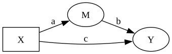

model.equations()

\begin{aligned} \beta_{M} &\sim \text{Normal}(mu=0,\, sigma=10) \\ \sigma_{M} &\sim \text{HalfNormal}(sigma=1) \\ \beta_{Y} &\sim \text{Normal}(mu=0,\, sigma=10) \\ \sigma_{Y} &\sim \text{HalfNormal}(sigma=1) \\[6pt] \mu_{M} &= \beta_{0,\,M} + a \cdot \mathrm{X} \\ \mathrm{M} &\sim \text{Normal}(\mu_{M},\, \sigma_{M}) \\ \mu_{Y} &= \beta_{0,\,Y} + b \cdot \mathrm{M} + c \cdot \mathrm{X} \\ \mathrm{Y} &\sim \text{Normal}(\mu_{Y},\, \sigma_{Y}) \\ indirect &\equiv a \cdot b \end{aligned}

equations() shows the structural equations and the prior distribution assigned to every parameter, including defaults you may not have thought about. The defaults are deliberately vague: Normal(0, 10) for regression coefficients and HalfNormal(1) for residual scales. These work out of the box, but domain knowledge almost always lets you do better.

3. Prior predictive check

A prior predictive check asks: if we generated data from our priors (without seeing real data), would it look remotely plausible?

ppc_default = model.sample_prior_predictive(draws=500, random_seed=42)

Sampling: [M, Y, beta_M, beta_Y, sigma_M, sigma_Y]

import matplotlib.pyplot as plt
import arviz as az

FIG_WIDTH = 7
FIG_HEIGHT = 3.5
COLOR_DEFAULT = "#1b9e77"
COLOR_CUSTOM = "#d95f02"

y_prior = ppc_default.prior["Y"].values.flatten()

fig, ax = plt.subplots(figsize=(FIG_WIDTH, FIG_HEIGHT))
x_kde, y_kde, _ = az.kde(y_prior)
ax.plot(x_kde, y_kde, color=COLOR_DEFAULT, lw=2, label="Prior predictive (defaults)")
ax.fill_between(x_kde, y_kde, alpha=0.6, color=COLOR_DEFAULT)
ax.axvline(
    df["Y"].mean(),
    color="black",
    linestyle="--",
    linewidth=1.5,
    label=f"Observed mean = {df['Y'].mean():.2f}",
)
ax.set_xlabel("Y")
ax.set_ylabel("Density")
ax.legend()
plt.tight_layout()
plt.show()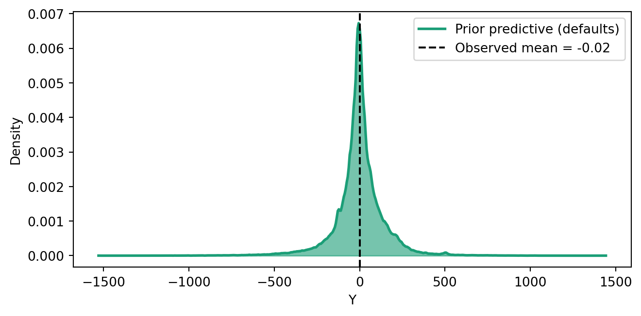

Figure 2: Prior predictive distribution of Y under default priors. The tails extend well beyond the observed data range, indicating the model considers extreme outcomes plausible.

The default priors generate Y values spanning a huge range. For this dataset, where Y lives roughly in [-2, 2], coefficients of \pm 10 are implausible. We can do better.

4. Refine priors

set_priors() merges overrides into the current configuration and recompiles. Only the parameters you specify change.

model.set_priors({
    "beta_M": Prior("Normal", mu=0, sigma=2),
    "beta_Y": Prior("Normal", mu=0, sigma=2),
    "sigma_M": Prior("HalfNormal", sigma=0.5),
    "sigma_Y": Prior("HalfNormal", sigma=0.5),
})

model.equations()

\begin{aligned} \beta_{M} &\sim \text{Normal}(mu=0,\, sigma=2) \\ \sigma_{M} &\sim \text{HalfNormal}(sigma=0.5) \\ \beta_{Y} &\sim \text{Normal}(mu=0,\, sigma=2) \\ \sigma_{Y} &\sim \text{HalfNormal}(sigma=0.5) \\[6pt] \mu_{M} &= \beta_{0,\,M} + a \cdot \mathrm{X} \\ \mathrm{M} &\sim \text{Normal}(\mu_{M},\, \sigma_{M}) \\ \mu_{Y} &= \beta_{0,\,Y} + b \cdot \mathrm{M} + c \cdot \mathrm{X} \\ \mathrm{Y} &\sim \text{Normal}(\mu_{Y},\, \sigma_{Y}) \\ indirect &\equiv a \cdot b \end{aligned}

Now re-check: do the refined priors generate plausible data?

ppc_custom = model.sample_prior_predictive(draws=500, random_seed=42)

Sampling: [M, Y, beta_M, beta_Y, sigma_M, sigma_Y]

y_default = ppc_default.prior["Y"].values.flatten()
y_custom = ppc_custom.prior["Y"].values.flatten()

fig, ax = plt.subplots(figsize=(FIG_WIDTH, FIG_HEIGHT))
x_kde, y_kde, _ = az.kde(y_default)
ax.plot(x_kde, y_kde, color=COLOR_DEFAULT, lw=2, label="Default priors")
ax.fill_between(x_kde, y_kde, alpha=0.45, color=COLOR_DEFAULT)
x_kde, y_kde, _ = az.kde(y_custom)
ax.plot(x_kde, y_kde, color=COLOR_CUSTOM, lw=2, label="Refined priors")
ax.fill_between(x_kde, y_kde, alpha=0.55, color=COLOR_CUSTOM)
ax.axvline(
    df["Y"].mean(),
    color="black",
    linestyle="--",
    linewidth=1.5,
    label=f"Observed mean = {df['Y'].mean():.2f}",
)
ax.set_xlabel("Y")
ax.set_ylabel("Density")
ax.legend()
plt.tight_layout()
plt.show()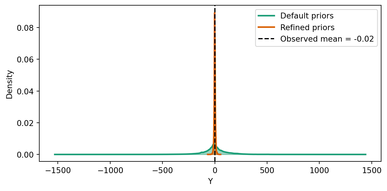

Figure 3: Prior predictive distributions under default (green) and refined (orange) priors. The refined priors concentrate mass in the plausible range.

The refined priors concentrate probability mass in the plausible range — much better. The model still allows coefficients up to \pm 4–6 (generous), but no longer considers coefficients of 10 or 20 as likely.

TipThis loop is cheap

sample_prior_predictive() draws from priors without MCMC — it runs in seconds. Iterate as many times as needed before committing to a full posterior fit.

5. Fit

With priors that generate plausible data, run MCMC.

model.fit(draws=500, tune=500, chains=4, random_seed=42)

NUTS[nutpie]: [beta_Y, sigma_M, beta_M, sigma_Y]

<xarray.DataTree>
Group: /
├── Group: /posterior
│       Dimensions:       (chain: 4, draw: 500, Y_predictors: 3, M_predictors: 2,
│                          mu_Y_dim_0: 500, mu_M_dim_0: 500)
│       Coordinates:
│         * chain         (chain) int64 32B 0 1 2 3
│         * draw          (draw) int64 4kB 0 1 2 3 4 5 6 ... 493 494 495 496 497 498 499
│         * Y_predictors  (Y_predictors) object 24B 'Intercept' 'M' 'X'
│         * M_predictors  (M_predictors) object 16B 'Intercept' 'X'
│         * mu_Y_dim_0    (mu_Y_dim_0) int64 4kB 0 1 2 3 4 5 ... 494 495 496 497 498 499
│         * mu_M_dim_0    (mu_M_dim_0) int64 4kB 0 1 2 3 4 5 ... 494 495 496 497 498 499
│       Data variables:
│           beta_Y        (chain, draw, Y_predictors) float64 48kB 0.01076 ... 0.3407
│           beta_M        (chain, draw, M_predictors) float64 32kB -0.01287 ... 0.5213
│           sigma_M       (chain, draw) float64 16kB 0.2867 0.3084 ... 0.2913 0.3228
│           sigma_Y       (chain, draw) float64 16kB 0.297 0.3052 ... 0.3113 0.3007
│           mu_Y          (chain, draw, mu_Y_dim_0) float64 8MB 0.5402 ... -0.8795
│           mu_M          (chain, draw, mu_M_dim_0) float64 8MB 0.1378 ... -0.7864
│       Attributes:
│           created_at:                 2026-08-07T10:16:08.501042+00:00
│           creation_library:           ArviZ
│           creation_library_version:   1.1.0
│           creation_library_language:  Python
│           sample_dims:                ['chain', 'draw']
│           inference_library:          nutpie
│           inference_library_version:  0.16.10
│           sampling_time:              0.0751340389251709
│           tuning_steps:               500
├── Group: /sample_stats
│       Dimensions:                   (chain: 4, draw: 500)
│       Coordinates:
│         * chain                     (chain) int64 32B 0 1 2 3
│         * draw                      (draw) int64 4kB 0 1 2 3 4 ... 495 496 497 498 499
│       Data variables: (12/20)
│           depth                     (chain, draw) uint64 16kB 2 3 3 2 2 ... 2 2 3 3 3
│           maxdepth_reached          (chain, draw) bool 2kB False False ... False False
│           step_size                 (chain, draw) float64 16kB 0.6706 0.652 ... 0.7469
│           transformation_update_id  (chain, draw) int64 16kB 0 0 0 0 0 0 ... 0 0 0 0 0
│           step_size_bar             (chain, draw) float64 16kB 0.7114 ... 0.7294
│           mean_tree_accept          (chain, draw) float64 16kB 0.5497 ... 0.9232
│           ...                        ...
│           fisher_distance           (chain, draw) float64 16kB 0.1828 0.2064 ... 0.304
│           transformation_index      (chain, draw) int64 16kB 420 420 420 ... 423 423
│           diverging                 (chain, draw) bool 2kB False False ... False False
│           divergence_draw           (chain, draw) uint64 16kB 0 0 0 0 0 ... 0 0 0 0 0
│           divergence_message        (chain, draw) object 16kB None None ... None None
│           divergence_energy_error   (chain, draw) float64 16kB nan nan nan ... nan nan
│       Attributes:
│           created_at:                  2026-08-07T10:16:08.495329+00:00
│           creation_library:            ArviZ
│           creation_library_version:    1.1.0
│           creation_library_language:   Python
│           sample_dims:                 ['chain', 'draw']
│           inference_library:           nutpie
│           inference_library_version:   0.16.10
│           inference_library_settings:  {"sampler": "nuts", "adaptation": "diag", "s...
├── Group: /constant_data
│       Dimensions:  (X_dim_0: 500)
│       Coordinates:
│         * X_dim_0  (X_dim_0) int64 4kB 0 1 2 3 4 5 6 7 ... 493 494 495 496 497 498 499
│       Data variables:
│           X        (X_dim_0) float64 4kB 0.3047 -1.04 0.7505 ... -0.3356 -1.991 -1.495
│       Attributes:
│           created_at:                 2026-08-07T10:16:08.498874+00:00
│           creation_library:           ArviZ
│           creation_library_version:   1.1.0
│           creation_library_language:  Python
│           inference_library:          pymc
│           inference_library_version:  6.0.1
│           sample_dims:                []
├── Group: /observed_data
│       Dimensions:  (M_dim_0: 500, Y_dim_0: 500)
│       Coordinates:
│         * M_dim_0  (M_dim_0) int64 4kB 0 1 2 3 4 5 6 7 ... 493 494 495 496 497 498 499
│         * Y_dim_0  (Y_dim_0) int64 4kB 0 1 2 3 4 5 6 7 ... 493 494 495 496 497 498 499
│       Data variables:
│           M        (M_dim_0) float64 4kB 0.5615 -0.2514 0.1594 ... -0.9562 -0.5004
│           Y        (Y_dim_0) float64 4kB 0.5228 -0.7319 0.2283 ... -1.149 -1.203
│       Attributes:
│           created_at:                 2026-08-07T10:16:08.500308+00:00
│           creation_library:           ArviZ
│           creation_library_version:   1.1.0
│           creation_library_language:  Python
│           inference_library:          pymc
│           inference_library_version:  6.0.1
│           sample_dims:                []
└── Group: /log_likelihood
        Dimensions:  (chain: 4, draw: 500, M_dim_0: 500, Y_dim_0: 500)
        Coordinates:
          * chain    (chain) int64 32B 0 1 2 3
          * draw     (draw) int64 4kB 0 1 2 3 4 5 6 7 ... 493 494 495 496 497 498 499
          * M_dim_0  (M_dim_0) int64 4kB 0 1 2 3 4 5 6 7 ... 493 494 495 496 497 498 499
          * Y_dim_0  (Y_dim_0) int64 4kB 0 1 2 3 4 5 6 7 ... 493 494 495 496 497 498 499
        Data variables:
            M        (chain, draw, M_dim_0) float64 8MB -0.7618 -0.1313 ... -0.1807
            Y        (chain, draw, Y_dim_0) float64 8MB 0.2933 0.05542 ... -0.2971
        Attributes:
            created_at:                 2026-08-07T10:16:08.574793+00:00
            creation_library:           ArviZ
            creation_library_version:   1.1.0
            creation_library_language:  Python
            inference_library:          pymc
            inference_library_version:  6.0.1
            sample_dims:                ['chain', 'draw']

xarray.DataTree

• /posterior(21)

  • Dimensions:
    • chain: 4
    • draw: 500
    • Y_predictors: 3
    • M_predictors: 2
    • mu_Y_dim_0: 500
    • mu_M_dim_0: 500
  • Coordinates: (6)
    • chain
      (chain)
      int64
      0 1 2 3

      array([0, 1, 2, 3])

    • draw
      (draw)
      int64
      0 1 2 3 4 5 ... 495 496 497 498 499

      array([  0,   1,   2, ..., 497, 498, 499], shape=(500,))

    • Y_predictors
      (Y_predictors)
      object
      'Intercept' 'M' 'X'

      array(['Intercept', 'M', 'X'], dtype=object)

    • M_predictors
      (M_predictors)
      object
      'Intercept' 'X'

      array(['Intercept', 'X'], dtype=object)

    • mu_Y_dim_0
      (mu_Y_dim_0)
      int64
      0 1 2 3 4 5 ... 495 496 497 498 499

      array([  0,   1,   2, ..., 497, 498, 499], shape=(500,))

    • mu_M_dim_0
      (mu_M_dim_0)
      int64
      0 1 2 3 4 5 ... 495 496 497 498 499

      array([  0,   1,   2, ..., 497, 498, 499], shape=(500,))

  • Data variables: (6)
    • beta_Y
      (chain, draw, Y_predictors)
      float64
      0.01076 0.7627 ... 0.7477 0.3407

      array([[[ 1.07647969e-02,  7.62670733e-01,  3.32045132e-01],[-2.54085229e-03,  7.70333451e-01,  3.27945166e-01],[-2.86542033e-02,  7.81223745e-01,  3.29531443e-01],...,[-1.35851519e-02,  8.01491141e-01,  3.27289625e-01],[ 1.10978272e-02,  8.14568070e-01,  3.34804849e-01],[ 3.21449310e-04,  7.97466930e-01,  2.99391834e-01]],[[ 2.18305834e-02,  7.51846753e-01,  3.42533453e-01],[ 1.22498965e-02,  7.95356083e-01,  2.99140300e-01],[ 2.40008745e-04,  7.72929566e-01,  2.96458165e-01],...,[ 8.53543925e-03,  7.19712858e-01,  3.58298645e-01],[ 2.07139516e-03,  7.19494066e-01,  3.64101088e-01],[-3.85835273e-03,  7.01527428e-01,  3.53872371e-01]],[[ 1.10407148e-02,  8.41034806e-01,  3.07787758e-01],[-4.59597499e-03,  8.06415372e-01,  2.92530900e-01],[ 3.07110595e-04,  8.35578069e-01,  3.02812284e-01],...,[ 7.21271575e-03,  6.68482006e-01,  3.70255701e-01],[ 2.15852306e-02,  7.25444008e-01,  3.89001217e-01],[-2.75692376e-03,  7.12053239e-01,  3.75935567e-01]],[[ 3.10603313e-03,  7.16109662e-01,  3.72967895e-01],[-1.16438660e-02,  7.42533695e-01,  3.43424229e-01],[-8.47101531e-03,  7.76162378e-01,  3.25252170e-01],...,[-2.36618608e-02,  8.36595888e-01,  2.88146908e-01],[-6.68692472e-03,  8.00497258e-01,  3.14397529e-01],[ 4.02545521e-03,  7.47745766e-01,  3.40668287e-01]]],shape=(4, 500, 3))

    • beta_M
      (chain, draw, M_predictors)
      float64
      -0.01287 0.4943 ... 0.5213

      array([[[-0.01286528,  0.4942967 ],[-0.04085626,  0.48797437],[-0.0056534 ,  0.4833568 ],...,[-0.03169383,  0.47797172],[-0.01150336,  0.49090596],[-0.02636293,  0.48325675]],[[-0.02186062,  0.48550732],[-0.00898273,  0.49574011],[-0.0044056 ,  0.50624451],...,[-0.03301761,  0.50603624],[-0.04487145,  0.51069751],[ 0.0178455 ,  0.4840204 ]],[[-0.00807051,  0.48735866],[ 0.00561976,  0.47138382],[ 0.01048487,  0.4938825 ],...,[-0.01529697,  0.48536657],[-0.01231856,  0.48472059],[-0.02317276,  0.52512768]],[[ 0.00196988,  0.49854098],[-0.01622771,  0.5022873 ],[-0.00218033,  0.4808261 ],...,[-0.01501806,  0.48687827],[-0.02111977,  0.47571014],[-0.00696941,  0.52132082]]], shape=(4, 500, 2))

    • sigma_M
      (chain, draw)
      float64
      0.2867 0.3084 ... 0.2913 0.3228

      array([[0.28673443, 0.30840533, 0.30271998, ..., 0.31168255, 0.29796817,0.31215691],[0.31787453, 0.29628095, 0.30532441, ..., 0.31266348, 0.30909843,0.29990921],[0.32211699, 0.32834179, 0.31886366, ..., 0.30355534, 0.29484921,0.30937458],[0.32264911, 0.29142772, 0.30906608, ..., 0.31171706, 0.2913249 ,0.32284295]], shape=(4, 500))

    • sigma_Y
      (chain, draw)
      float64
      0.297 0.3052 ... 0.3113 0.3007

      array([[0.29701675, 0.30524162, 0.33113801, ..., 0.28974977, 0.3248537 ,0.30129386],[0.30245428, 0.29112183, 0.29608058, ..., 0.31309108, 0.3122058 ,0.3090885 ],[0.31597652, 0.31970801, 0.31149414, ..., 0.29604921, 0.29749568,0.33030127],[0.30988123, 0.3026712 , 0.30127724, ..., 0.29950416, 0.31130267,0.30065229]], shape=(4, 500))

    • mu_Y
      (chain, draw, mu_Y_dim_0)
      float64
      0.5402 -0.5263 ... -1.389 -0.8795

      array([[[ 0.54019736, -0.52632017,  0.38150409, ..., -0.20092529,-1.37952265, -0.86730672],[ 0.52994513, -0.5372886 ,  0.36634291, ..., -0.21386223,-1.39199295, -0.87831713],[ 0.51043023, -0.56778988,  0.3431557 , ..., -0.24193948,-1.43167733, -0.91225161],...,[ 0.53619666, -0.55548533,  0.35977262, ..., -0.22878221,-1.43152445, -0.9039728 ],[ 0.57051257, -0.54190609,  0.39217963, ..., -0.20834036,-1.43430673, -0.8970693 ],[ 0.53934266, -0.51155364,  0.35210191, ..., -0.20498392,-1.35823074, -0.84634358]],[[ 0.54838127, -0.52344052,  0.39871571, ..., -0.19195665,-1.3789875 , -0.86650524],[ 0.55000918, -0.49883286,  0.36350516, ..., -0.19269359,-1.34378319, -0.83298279],[ 0.52458913, -0.50241452,  0.34590809, ..., -0.20085536,-1.32900973, -0.82976039],...[ 0.4954001 , -0.54592814,  0.39161523, ..., -0.20491999,-1.36908372, -0.88085347],[ 0.54746984, -0.565373  ,  0.42913403, ..., -0.20432628,-1.44649575, -0.92301068],[ 0.51162721, -0.57276015,  0.39285251, ..., -0.22252328,-1.43202271, -0.92111809]],[[ 0.51886362, -0.5648308 ,  0.39713489, ..., -0.21619757,-1.42413033, -0.91284814],[ 0.50994881, -0.55549972,  0.36442541, ..., -0.22450584,-1.40533039, -0.89665116],[ 0.52646741, -0.5418837 ,  0.35932081, ..., -0.21965482,-1.39813535, -0.88313792],...,[ 0.53390441, -0.53368086,  0.32591626, ..., -0.23033687,-1.39724171, -0.87309534],[ 0.53860836, -0.53492963,  0.35683755, ..., -0.21742666,-1.39801016, -0.87730277],[ 0.52770502, -0.53827477,  0.37885724, ..., -0.20859674,-1.38915817, -0.87946969]]], shape=(4, 500, 500))

    • mu_M
      (chain, draw, mu_M_dim_0)
      float64
      0.1378 -0.5269 ... -1.045 -0.7864

      array([[[ 0.13775536, -0.526926  ,  0.35808027, ..., -0.1787549 ,-0.99691709, -0.75186893],[ 0.10783786, -0.54834185,  0.32534469, ..., -0.20462405,-1.01232148, -0.77040762],[ 0.14163367, -0.50833679,  0.35708229, ..., -0.1678715 ,-0.96792592, -0.72830122],...,[ 0.11395232, -0.52877683,  0.32700062, ..., -0.19210466,-0.98324567, -0.74629063],[ 0.13808407, -0.52203776,  0.35689761, ..., -0.17625502,-0.98880484, -0.74543764],[ 0.12089366, -0.52894226,  0.33629768, ..., -0.18854745,-0.98843626, -0.74886116]],[[ 0.12608175, -0.52678052,  0.34248893, ..., -0.18480046,-0.98841442, -0.7477236 ],[ 0.14207774, -0.52454457,  0.36304603, ..., -0.17535677,-0.9959081 , -0.75014436],[ 0.14985575, -0.53089185,  0.3755062 , ..., -0.17430499,-1.01224325, -0.76127194],...[ 0.13260251, -0.52007049,  0.34894695, ..., -0.17818957,-0.98157057, -0.74094952],[ 0.13538408, -0.51642027,  0.35144058, ..., -0.17499436,-0.97730612, -0.73700532],[ 0.13684261, -0.5692972 ,  0.37090994, ..., -0.19940948,-1.06860324, -0.80827059]],[[ 0.15388383, -0.51650481,  0.37610056, ..., -0.16534414,-0.99053147, -0.7433792 ],[ 0.13682781, -0.53859852,  0.36071439, ..., -0.18479903,-1.01618729, -0.76717778],[ 0.14433559, -0.50223183,  0.35865619, ..., -0.16354911,-0.95941469, -0.72104459],...,[ 0.13334207, -0.52136373,  0.35036032, ..., -0.178418  ,-0.98430117, -0.7429307 ],[ 0.12383723, -0.51585076,  0.33587747, ..., -0.1807716 ,-0.96816923, -0.73233538],[ 0.15188595, -0.54913478,  0.38425643, ..., -0.18192852,-1.04482116, -0.78637575]]], shape=(4, 500, 500))

  • Attributes: (9)

    created_at :

    2026-08-07T10:16:08.501042+00:00

    creation_library :

    ArviZ

    creation_library_version :

    1.1.0

    creation_library_language :

    Python

    sample_dims :

    ['chain', 'draw']

    inference_library :

    nutpie

    inference_library_version :

    0.16.10

    sampling_time :

    0.0751340389251709

    tuning_steps :

    500

  /sample_stats(30)

  • Dimensions:
    • chain: 4
    • draw: 500
  • Coordinates: (2)
    • chain
      (chain)
      int64
      0 1 2 3

      array([0, 1, 2, 3])

    • draw
      (draw)
      int64
      0 1 2 3 4 5 ... 495 496 497 498 499

      array([  0,   1,   2, ..., 497, 498, 499], shape=(500,))

  • Data variables: (20)
    • depth
      (chain, draw)
      uint64
      2 3 3 2 2 3 3 3 ... 3 2 2 2 2 3 3 3

      array([[2, 3, 3, ..., 2, 3, 3],[3, 2, 2, ..., 3, 2, 3],[2, 2, 2, ..., 3, 3, 3],[3, 3, 3, ..., 3, 3, 3]], shape=(4, 500), dtype=uint64)

    • maxdepth_reached
      (chain, draw)
      bool
      False False False ... False False

      array([[False, False, False, ..., False, False, False],[False, False, False, ..., False, False, False],[False, False, False, ..., False, False, False],[False, False, False, ..., False, False, False]], shape=(4, 500))

    • step_size
      (chain, draw)
      float64
      0.6706 0.652 ... 0.7694 0.7469

      array([[0.67057228, 0.65195616, 0.77112801, ..., 0.76178533, 0.67596484,0.71752898],[0.75601066, 0.75722582, 0.74305741, ..., 0.69965173, 0.66741869,0.69866054],[0.72839576, 0.71964551, 0.73718868, ..., 0.66103483, 0.70338883,0.71322617],[0.70741831, 0.70992622, 0.76723317, ..., 0.70443251, 0.76944747,0.7469221 ]], shape=(4, 500))

    • transformation_update_id
      (chain, draw)
      int64
      0 0 0 0 0 0 0 0 ... 0 0 0 0 0 0 0 0

      array([[0, 0, 0, ..., 0, 0, 0],[0, 0, 0, ..., 0, 0, 0],[0, 0, 0, ..., 0, 0, 0],[0, 0, 0, ..., 0, 0, 0]], shape=(4, 500))

    • step_size_bar
      (chain, draw)
      float64
      0.7114 0.7114 ... 0.7294 0.7294

      array([[0.71144765, 0.71144765, 0.71144765, ..., 0.71144765, 0.71144765,0.71144765],[0.71115503, 0.71115503, 0.71115503, ..., 0.71115503, 0.71115503,0.71115503],[0.70007417, 0.70007417, 0.70007417, ..., 0.70007417, 0.70007417,0.70007417],[0.72939232, 0.72939232, 0.72939232, ..., 0.72939232, 0.72939232,0.72939232]], shape=(4, 500))

    • mean_tree_accept
      (chain, draw)
      float64
      0.5497 0.8711 ... 0.9847 0.9232

      array([[0.54966438, 0.8711053 , 0.7623904 , ..., 0.5320438 , 0.59168233,0.98914599],[0.93278329, 0.33615981, 0.47758987, ..., 0.71337614, 0.91671128,0.71827881],[0.92648104, 0.76910875, 1.        , ..., 0.72565876, 0.57972232,0.82794381],[0.69619888, 0.57202   , 0.90496205, ..., 0.82845187, 0.98470686,0.92318892]], shape=(4, 500))

    • mean_tree_accept_sym
      (chain, draw)
      float64
      0.6409 0.9196 ... 0.9807 0.9373

      array([[0.6409139 , 0.91959764, 0.86033802, ..., 0.69058978, 0.72401725,0.82834969],[0.96149167, 0.32814395, 0.61569345, ..., 0.82192968, 0.93365449,0.82715793],[0.90862347, 0.8404893 , 0.84470778, ..., 0.82697628, 0.70225143,0.73894523],[0.81439094, 0.65945113, 0.94538709, ..., 0.90252049, 0.98072319,0.93727762]], shape=(4, 500))

    • n_steps
      (chain, draw)
      uint64
      3 7 7 3 3 7 7 7 ... 7 3 3 7 3 7 7 7

      array([[3, 7, 7, ..., 3, 7, 7],[7, 3, 3, ..., 7, 3, 7],[3, 3, 3, ..., 7, 7, 7],[7, 7, 7, ..., 7, 7, 7]], shape=(4, 500), dtype=uint64)

    • max_energy_error
      (chain, draw)
      float64
      -1.741 -0.349 ... 0.08591 -0.2912

      array([[-1.74146289, -0.3489789 , -0.46586572, ..., -0.87911625,-1.2700329 ,  0.60881441],[-0.16332563, -6.73898683, -1.52347952, ..., -0.57879273,-0.17599256, -0.63424361],[-0.24917557, -0.55285476,  0.54781087, ..., -0.78489267,-1.25589682,  0.96714543],[-0.5706229 , -1.48717163, -0.22355672, ..., -0.3711378 ,0.0859072 , -0.29115099]], shape=(4, 500))

    • tuning
      (chain, draw)
      bool
      False False False ... False False

      array([[False, False, False, ..., False, False, False],[False, False, False, ..., False, False, False],[False, False, False, ..., False, False, False],[False, False, False, ..., False, False, False]], shape=(4, 500))

    • index_in_trajectory
      (chain, draw)
      int64
      -2 3 3 2 2 7 -5 ... -2 -2 2 5 2 -4

      array([[-2,  3,  3, ...,  3, -3, -3],[-3,  2, -1, ...,  4,  1,  5],[-2, -1, -1, ...,  3,  1,  3],[ 3, -5, -3, ...,  5,  2, -4]], shape=(4, 500))

    • logp
      (chain, draw)
      float64
      -245.5 -244.8 ... -245.7 -245.7

      array([[-245.53516896, -244.82860616, -248.12669256, ..., -247.23353851,-247.10597649, -244.95449266],[-245.42756681, -246.20529829, -246.48169556, ..., -245.03697   ,-246.54433854, -247.23228355],[-246.83495476, -249.77754594, -246.40313325, ..., -246.47451268,-249.12867919, -248.72335065],[-245.81016295, -244.22050058, -243.94636968, ..., -246.40562319,-245.72817735, -245.72977193]], shape=(4, 500))

    • energy
      (chain, draw)
      float64
      222.2 222.5 223.8 ... 221.8 220.7

      array([[222.20921558, 222.45551295, 223.78856937, ..., 223.93156081,224.88366834, 221.42841684],[220.26080367, 228.08412925, 222.58487832, ..., 224.69781181,220.13457201, 225.21128506],[220.59298024, 225.36551489, 224.81191223, ..., 223.73458786,224.85280322, 226.40356298],[220.38555309, 223.25583637, 219.55403054, ..., 221.60511984,221.846919  , 220.74097799]], shape=(4, 500))

    • energy_error
      (chain, draw)
      float64
      -0.03683 -0.08105 ... 0.03695

      array([[-0.03682698, -0.08104989,  0.35606038, ...,  0.53086835,0.55085051, -0.59264492],[ 0.00970311, -0.06485983,  0.78574246, ..., -0.00287829,0.17599256,  0.24870883],[ 0.24917557,  0.31194588, -0.54781087, ...,  0.36892797,0.80012294, -0.48472331],[ 0.23978228, -0.27576042, -0.03567402, ...,  0.17535671,0.03241132,  0.03694629]], shape=(4, 500))

    • fisher_distance
      (chain, draw)
      float64
      0.1828 0.2064 0.422 ... 1.553 0.304

      array([[ 0.18277297,  0.2064103 ,  0.42195761, ...,  2.79538148,5.01833825,  4.27321758],[ 0.15728232,  4.76280354, 11.38727717, ...,  1.72956137,2.22039739,  4.43087411],[ 5.91713721,  4.30745522,  4.11111687, ...,  8.91222057,14.29523536,  4.37421022],[ 3.87418792,  0.41154997,  0.29496475, ...,  6.21609141,1.55304657,  0.30403622]], shape=(4, 500))

    • transformation_index
      (chain, draw)
      int64
      420 420 420 420 ... 423 423 423 423

      array([[420, 420, 420, ..., 420, 420, 420],[423, 423, 423, ..., 423, 423, 423],[423, 423, 423, ..., 423, 423, 423],[423, 423, 423, ..., 423, 423, 423]], shape=(4, 500))

    • diverging
      (chain, draw)
      bool
      False False False ... False False

      array([[False, False, False, ..., False, False, False],[False, False, False, ..., False, False, False],[False, False, False, ..., False, False, False],[False, False, False, ..., False, False, False]], shape=(4, 500))

    • divergence_draw
      (chain, draw)
      uint64
      0 0 0 0 0 0 0 0 ... 0 0 0 0 0 0 0 0

      array([[0, 0, 0, ..., 0, 0, 0],[0, 0, 0, ..., 0, 0, 0],[0, 0, 0, ..., 0, 0, 0],[0, 0, 0, ..., 0, 0, 0]], shape=(4, 500), dtype=uint64)

    • divergence_message
      (chain, draw)
      object
      None None None ... None None None

      array([[None, None, None, ..., None, None, None],[None, None, None, ..., None, None, None],[None, None, None, ..., None, None, None],[None, None, None, ..., None, None, None]],shape=(4, 500), dtype=object)

    • divergence_energy_error
      (chain, draw)
      float64
      nan nan nan nan ... nan nan nan nan

      array([[nan, nan, nan, ..., nan, nan, nan],[nan, nan, nan, ..., nan, nan, nan],[nan, nan, nan, ..., nan, nan, nan],[nan, nan, nan, ..., nan, nan, nan]], shape=(4, 500))

  • Attributes: (8)

    created_at :

    2026-08-07T10:16:08.495329+00:00

    creation_library :

    ArviZ

    creation_library_version :

    1.1.0

    creation_library_language :

    Python

    sample_dims :

    ['chain', 'draw']

    inference_library :

    nutpie

    inference_library_version :

    0.16.10

    inference_library_settings :

    {"sampler": "nuts", "adaptation": "diag", "settings": {"num_tune": 500, "num_draws": 500, "maxdepth": 10, "mindepth": 0, "store_gradient": false, "store_unconstrained": false, "store_transformed": false, "max_energy_error": 1000.0, "store_divergences": false, "adapt_options": {"step_size_settings": {"target_accept": 0.8, "initial_step": 0.1, "jitter": 0.1, "adapt_options": {"method": "DualAverage", "dual_average": {"k": 0.75, "t0": 10.0, "gamma": 0.05, "max_step_size": 3.141592653589793}, "adam": {"beta1": 0.9, "beta2": 0.999, "epsilon": 1e-08, "learning_rate": 0.05}}}, "mass_matrix_options": {"store_mass_matrix": false, "use_grad_based_estimate": true}, "early_window": 0.3, "step_size_window": 0.15, "mass_matrix_switch_freq": 80, "early_mass_matrix_switch_freq": 10, "mass_matrix_update_freq": 1, "mass_matrix_window_growth": 1.5}, "check_turning": true, "target_integration_time": null, "trajectory_kind": "Euclidean", "num_chains": 4, "seed": 534082709, "extra_doublings": 0}}

  /constant_data(9)

  • Dimensions:
    • X_dim_0: 500
  • Coordinates: (1)
    • X_dim_0
      (X_dim_0)
      int64
      0 1 2 3 4 5 ... 495 496 497 498 499

      array([  0,   1,   2, ..., 497, 498, 499], shape=(500,))

  • Data variables: (1)
    • X
      (X_dim_0)
      float64
      0.3047 -1.04 ... -1.991 -1.495

      array([ 3.04717080e-01, -1.03998411e+00,  7.50451196e-01,  9.40564716e-01,-1.95103519e+00, -1.30217951e+00,  1.27840403e-01, -3.16242592e-01,-1.68011575e-02, -8.53043928e-01,  8.79397975e-01,  7.77791935e-01,6.60306976e-02,  1.12724121e+00,  4.67509342e-01, -8.59292463e-01,3.68750784e-01, -9.58882601e-01,  8.78450301e-01, -4.99259110e-02,-1.84862364e-01, -6.80929544e-01,  1.22254134e+00, -1.54529482e-01,-4.28327822e-01, -3.52133550e-01,  5.32309186e-01,  3.65444064e-01,4.12732612e-01,  4.30821003e-01,  2.14164760e+00, -4.06415016e-01,-5.12242729e-01, -8.13772728e-01,  6.15979423e-01,  1.12897229e+00,-1.13947458e-01, -8.40156477e-01, -8.24481216e-01,  6.50592788e-01,7.43254171e-01,  5.43154268e-01, -6.65509707e-01,  2.32161323e-01,1.16685809e-01,  2.18688597e-01,  8.71428778e-01,  2.23595549e-01,6.78913563e-01,  6.75790695e-02,  2.89119399e-01,  6.31288226e-01,-1.45715582e+00, -3.19671216e-01, -4.70372654e-01, -6.38877848e-01,-2.75142251e-01,  1.49494131e+00, -8.65831116e-01,  9.68278355e-01,-1.68286977e+00, -3.34885030e-01,  1.62753065e-01,  5.86222331e-01,7.11226580e-01,  7.93347235e-01, -3.48725072e-01, -4.62351793e-01,8.57975881e-01, -1.91304325e-01, -1.27568632e+00, -1.13328721e+00,-9.19452286e-01,  4.97160744e-01,  1.42425736e-01,  6.90485354e-01,-4.27252646e-01,  1.58539691e-01,  6.25590394e-01, -3.09346540e-01,...9.21266584e-02, -8.37398224e-01, -5.94400352e-01, -1.48053651e+00,-8.88133854e-01, -3.58016688e-01,  8.03585019e-01,  1.72076983e+00,-1.38218152e+00,  3.92827468e-01, -1.04054394e+00,  4.74697088e-01,-1.31086651e-01, -1.83090583e+00,  9.28296992e-01, -6.05000713e-01,-5.33900238e-01, -1.06975241e+00, -6.54283277e-01,  4.27890441e-01,-1.89244341e-01,  3.28662002e-01,  3.61921854e-01,  1.32066166e+00,-3.42786151e-01, -1.47685782e+00,  1.06722242e+00, -3.31488172e-01,1.11459244e+00,  3.83377113e-01, -1.31137530e-01,  3.48775894e-01,1.95101256e+00,  2.07698053e+00,  6.93811351e-02,  1.60190593e-01,1.07624016e+00, -8.45661033e-01,  3.33070373e-01, -2.58628480e-02,3.13908211e-01, -8.33368806e-01, -1.58956749e+00, -2.07298344e+00,-1.11738411e+00, -4.58675285e-01, -2.93191587e-01,  1.93723116e+00,1.10599337e+00, -9.62091116e-01,  3.47708452e-01, -4.07078236e-01,-2.84363838e-01,  1.85325649e-01,  6.19171117e-01, -3.39258484e-01,1.06385153e+00, -1.14193823e+00,  6.33906236e-03,  2.59767373e+00,2.23079743e-01,  1.43321451e+00,  9.15201782e-02,  5.80777095e-01,-5.67831944e-02, -1.70407581e-01, -7.79482397e-01,  4.30301359e-01,-8.51537189e-01,  6.65585236e-01,  1.08528700e+00,  3.66531407e-01,-2.86248734e-01,  4.53965579e-01, -3.08673056e-01,  9.35547125e-01,-1.83140608e+00, -3.35607368e-01, -1.99081200e+00, -1.49506083e+00])

  • Attributes: (7)

    created_at :

    2026-08-07T10:16:08.498874+00:00

    creation_library :

    ArviZ

    creation_library_version :

    1.1.0

    creation_library_language :

    Python

    inference_library :

    pymc

    inference_library_version :

    6.0.1

    sample_dims :

    []

  /observed_data(11)

  • Dimensions:
    • M_dim_0: 500
    • Y_dim_0: 500
  • Coordinates: (2)
    • M_dim_0
      (M_dim_0)
      int64
      0 1 2 3 4 5 ... 495 496 497 498 499

      array([  0,   1,   2, ..., 497, 498, 499], shape=(500,))

    • Y_dim_0
      (Y_dim_0)
      int64
      0 1 2 3 4 5 ... 495 496 497 498 499

      array([  0,   1,   2, ..., 497, 498, 499], shape=(500,))

  • Data variables: (2)
    • M
      (M_dim_0)
      float64
      0.5615 -0.2514 ... -0.9562 -0.5004

      array([ 0.56151721, -0.25143656,  0.15938153,  0.01953132, -1.86487625,-0.81413841,  0.79004471, -0.02765601, -0.17627226, -0.2869979 ,-0.02858852,  0.29969896,  0.06285859,  0.53779041,  0.47099651,-0.32625266,  0.3848732 , -0.68595299,  0.70856977,  0.46371813,-0.38347604, -0.60677347,  1.01200597, -0.13466794,  0.20698251,-0.30882749,  0.70266827,  0.22216778,  0.28383495,  0.68482591,0.96229266, -0.48554414, -0.39069063, -0.27118618, -0.16173801,0.75572742, -0.21860512, -0.07573444, -1.1305187 ,  0.08932666,-0.13431336,  0.02370829, -0.25845508,  0.06231267, -0.01767037,0.06158884,  0.49673086, -0.19076304,  0.55151167,  0.23258933,0.26007108,  0.48260415, -0.63965251,  0.45068638, -0.26131458,-0.41156389, -0.3636294 ,  0.43779185, -0.80625709,  0.21749998,-0.862639  , -0.06715398,  0.09671915,  0.06345058,  0.62566866,0.61849742, -0.22225703, -0.42705074,  0.59351632, -0.03926009,-1.07228134, -0.58703768, -0.3811154 , -0.02132806,  0.12816589,-0.09120407,  0.18722951,  0.45365484,  0.23704   , -0.04563697,-0.49458897, -0.67786727, -0.2696606 , -0.51250885, -0.38360088,0.8426752 , -0.58768559, -0.24499196,  0.31100784,  0.70660043,-0.03401974,  0.02546809,  0.3347405 , -0.53538685, -1.22798798,-0.85063822, -0.81752633, -0.25484303,  0.27238503, -0.98522815,...0.0271018 ,  0.129154  ,  0.36603149,  0.27961225,  0.07392139,0.48517006, -0.12640052,  0.03165459, -0.97555431, -0.97110972,-0.96661945, -1.04769807, -0.17245759,  0.18806664,  0.15377951,0.44614737,  0.97549928,  0.82266709,  0.37445965,  0.11255342,-0.04930864, -0.67880069, -0.26143242, -0.91170302, -0.49391428,0.38564412,  0.35087657,  0.98452261, -0.76077156,  0.21912772,-0.51846697,  0.37184576,  0.28404894, -0.42123471,  0.55703452,-0.12563629, -0.61220947, -0.56123923, -0.0450548 ,  0.47373581,-0.03113925,  0.43024919,  0.32819094,  1.02042271, -0.08458533,-0.8451384 ,  0.63436359, -1.0449224 ,  0.67216194, -0.90283529,-0.58260779,  0.30991853,  1.11876508,  0.68976163, -0.17894004,0.49125759,  0.39291104,  0.25004558,  0.16595923,  0.10947943,0.64201643, -0.37737627, -1.09548694, -1.06940995, -0.56937528,-0.63876014, -0.22334541,  0.74595795,  0.83030401, -0.470662  ,0.0890155 , -0.2353937 , -0.07524531,  0.27770708,  0.00967189,-0.48210553,  0.86332953, -0.69467017, -0.4218831 ,  1.43198068,0.25055081,  0.25739268,  0.1146046 ,  0.51106348,  0.08392434,0.10439065, -0.81102193,  0.31446273, -0.51655452,  0.18795557,0.80381019,  0.62704806,  0.39518665,  0.62142515, -0.18725678,0.57358961, -0.68565618, -0.1314503 , -0.95617674, -0.50040448])

    • Y
      (Y_dim_0)
      float64
      0.5228 -0.7319 ... -1.149 -1.203

      array([ 0.5228441 , -0.73193056,  0.22829866,  0.48796759, -2.07631357,-0.93990158,  0.87141166, -0.22945003,  0.08081629, -0.37185872,-0.12949535,  0.90578819, -0.08012734,  0.27187609,  0.2035369 ,-0.82510342,  0.43417579, -0.91858232,  0.72934132,  0.54190732,-0.26027693, -0.59488328,  1.29931571,  0.03074721, -0.59529834,-0.46203353,  0.06776435,  0.29818542,  0.34949785,  0.99076671,1.76861872, -0.4495273 , -0.61633364, -0.31553243, -0.10297187,0.94285583,  0.08677256, -0.4799659 , -0.91005573,  0.46985958,-0.17091198,  0.47408115, -0.19684708,  0.1500763 , -0.20782759,-0.14288416,  0.49751455,  0.07724657,  0.35819586,  0.33759886,-0.07773397,  0.51424921, -0.91597443,  0.99818678, -0.76335816,-0.0793101 , -0.32849347,  0.92206745, -0.86925064,  0.59790154,-1.24107766,  0.28202636, -0.0107401 ,  0.56629754,  0.52059277,0.71472655, -0.60401191, -0.34383901,  1.1657436 , -0.11200622,-1.29959668, -1.1440014 , -0.6495158 , -0.34575251, -0.12860297,0.20221817,  0.41731177,  1.25324904,  0.20133359,  0.30127651,-0.18551286, -0.78624589, -0.1948663 , -0.50595351, -0.63251388,0.69773196, -1.03040207, -0.65533289,  0.58900373,  0.61622967,-0.00642693, -0.00661948,  0.37928258, -0.39811576, -1.68540719,-0.74675643, -0.5770753 , -0.35468147,  0.62993934, -0.68723823,...0.32255724,  0.0651606 ,  0.47776288, -0.04192924,  0.04129187,0.51678559, -0.05961101,  0.46970383, -1.38099997, -1.01186953,-1.3436058 , -0.86932374, -0.81182453,  0.75356468,  0.44793062,0.16060728,  1.77594675,  1.3550866 ,  0.57016804,  0.50452516,-0.07697676, -0.85708267, -0.27030686, -0.75316749, -0.60717731,-0.0723228 ,  0.76910488,  1.58019426, -0.82687384,  0.51680009,-0.80821519,  0.16118899, -0.07254488, -1.37689849,  0.7952013 ,-0.30704388, -0.78193396, -1.65660275, -0.60652406,  0.84360798,-0.2810725 ,  0.55097546, -0.04607632,  1.64414831, -0.21371241,-1.03215595,  1.52539153, -0.48045234,  0.7801376 , -0.78522115,-0.60309099,  0.50553706,  1.44874859,  1.05633022,  0.31781668,0.40680029,  1.32707761, -0.02643908,  0.76828401,  0.18702052,0.89667378, -0.76929497, -1.60938757, -1.33951121, -0.49414948,-0.63653375, -0.65255181,  0.7698582 ,  0.5679003 , -1.19544357,0.20837054,  0.02707475, -0.14953014, -0.40036106,  0.13626071,-0.53630167,  1.63861871, -1.33545898, -0.45280804,  2.43664246,0.40235808,  0.80487241,  0.15351507,  0.68206697,  0.28338737,-0.21045565, -0.61924469, -0.03124032, -0.57019438,  0.40366232,0.78374632,  0.60479229,  0.04351265,  0.3118194 , -0.34849176,0.40833924, -1.00110753, -0.5508681 , -1.14859188, -1.20328555])

  • Attributes: (7)

    created_at :

    2026-08-07T10:16:08.500308+00:00

    creation_library :

    ArviZ

    creation_library_version :

    1.1.0

    creation_library_language :

    Python

    inference_library :

    pymc

    inference_library_version :

    6.0.1

    sample_dims :

    []

  /log_likelihood(13)

  • Dimensions:
    • chain: 4
    • draw: 500
    • M_dim_0: 500
    • Y_dim_0: 500
  • Coordinates: (4)
    • chain
      (chain)
      int64
      0 1 2 3

      array([0, 1, 2, 3])

    • draw
      (draw)
      int64
      0 1 2 3 4 5 ... 495 496 497 498 499

      array([  0,   1,   2, ..., 497, 498, 499], shape=(500,))

    • M_dim_0
      (M_dim_0)
      int64
      0 1 2 3 4 5 ... 495 496 497 498 499

      array([  0,   1,   2, ..., 497, 498, 499], shape=(500,))

    • Y_dim_0
      (Y_dim_0)
      int64
      0 1 2 3 4 5 ... 495 496 497 498 499

      array([  0,   1,   2, ..., 497, 498, 499], shape=(500,))

  • Data variables: (2)
    • M
      (chain, draw, M_dim_0)
      float64
      -0.7618 -0.1313 ... 0.174 -0.1807

      array([[[-7.61818622e-01, -1.31291286e-01,  9.01556583e-02, ...,3.16651582e-01,  3.20166375e-01, -5.42991818e-02],[-8.24590739e-01, -2.06004677e-01,  1.12608138e-01, ...,2.29254515e-01,  2.40830991e-01, -1.25832067e-01],[-6.85926017e-01, -8.40862581e-02,  6.27509219e-02, ...,2.68770881e-01,  2.75255326e-01, -7.36813831e-03],...,[-7.84164622e-01, -1.49055134e-01,  1.02223648e-01, ...,2.27896367e-01,  2.43060268e-01, -6.43495357e-02],[-7.17887537e-01, -1.20542423e-01,  7.21274789e-02, ...,2.80524882e-01,  2.85834728e-01, -4.62970290e-02],[-7.50918972e-01, -1.49844646e-01,  8.47057582e-02, ...,2.28582410e-01,  2.39970773e-01, -7.14456959e-02]],[[-7.11063116e-01, -1.47994065e-01,  6.12508595e-02, ...,2.13075884e-01,  2.22017372e-01, -7.55131859e-02],[-7.04568501e-01, -1.27337317e-01,  6.12469551e-02, ...,2.86528162e-01,  2.88517156e-01, -5.77449048e-02],[-6.41481661e-01, -1.51420735e-01,  1.69142420e-02, ...,2.57591715e-01,  2.50582023e-01, -9.75530016e-02],...2.61399002e-01,  2.69753764e-01, -4.07164193e-02],[-7.42032424e-01, -1.01486474e-01,  9.02043331e-02, ...,2.91447617e-01,  2.99784979e-01, -1.96078775e-02],[-6.87871419e-01, -2.73541959e-01,  2.05212224e-02, ...,2.30137327e-01,  1.88234453e-01, -2.40872046e-01]],[[-5.85832502e-01, -1.25210334e-01, -1.33299690e-02, ...,2.06733755e-01,  2.06582677e-01, -7.12996953e-02],[-7.47795833e-01, -1.71444950e-01,  7.53878090e-02, ...,2.97269257e-01,  2.92823372e-01, -1.04955009e-01],[-6.55736819e-01, -7.39733504e-02,  4.74013844e-02, ...,2.49868470e-01,  2.55206775e-01,  4.40030364e-04],...,[-6.96670246e-01, -1.28202152e-01,  5.90403231e-02, ...,2.35369479e-01,  2.42650621e-01, -5.59470032e-02],[-8.14191498e-01, -9.75153396e-02,  1.30857255e-01, ...,3.00046372e-01,  3.13530324e-01, -2.52952903e-03],[-5.93307887e-01, -2.13496972e-01, -3.09372544e-02, ...,1.99427275e-01,  1.73955213e-01, -1.80661803e-01]]],shape=(4, 500, 500))

    • Y
      (chain, draw, Y_dim_0)
      float64
      0.2933 0.05542 ... -0.03726 -0.2971

      array([[[ 0.29332144,  0.0554219 ,  0.1619961 , ..., -0.39904017,-0.00722556, -0.34475368],[ 0.26744249,  0.06440464,  0.16544994, ..., -0.34176407,-0.05021395, -0.29900206],[ 0.1855788 ,  0.06342888,  0.12612714, ..., -0.24889779,-0.17913403, -0.19994244],...,[ 0.31873722,  0.13438458,  0.21685451, ..., -0.29802838,-0.15694982, -0.21374984],[ 0.19467575,  0.03435622,  0.07819368, ..., -0.35044433,-0.18133458, -0.23883213],[ 0.2792314 ,  0.01323199,  0.19630909, ..., -0.37821684,0.03866513, -0.42102298]],[[ 0.27332215,  0.03930046,  0.1181502 , ..., -0.4271985 ,-0.0132476 , -0.34304517],[ 0.31072138, -0.00547558,  0.20722605, ..., -0.44177509,0.09030334, -0.4938987 ],[ 0.29816772, -0.00226769,  0.21929283, ..., -0.40055853,0.11252902, -0.49758912],...[ 0.29399433,  0.10092186,  0.14613028, ..., -0.38446274,0.02094166, -0.29479633],[ 0.28999106,  0.13669237,  0.06554603, ..., -0.38503631,-0.20795596, -0.15037243],[ 0.18823494,  0.07270036,  0.06471334, ..., -0.30528274,-0.17935442, -0.17607961]],[[ 0.25254515,  0.1072388 ,  0.10420139, ..., -0.33056817,-0.14268787, -0.18659485],[ 0.27526209,  0.10627617,  0.17503159, ..., -0.30516691,-0.08358779, -0.23701008],[ 0.28071354,  0.08182906,  0.18622164, ..., -0.32351451,-0.0622423 , -0.28381034],...,[ 0.28600657,  0.06761517,  0.23357302, ..., -0.2859823 ,-0.05793166, -0.32101636],[ 0.2467689 ,  0.04781569,  0.1628052 , ..., -0.32559424,-0.07291625, -0.30021785],[ 0.28273163,  0.07541782,  0.15747548, ..., -0.36514825,-0.03725596, -0.29714999]]], shape=(4, 500, 500))

  • Attributes: (7)

    created_at :

    2026-08-07T10:16:08.574793+00:00

    creation_library :

    ArviZ

    creation_library_version :

    1.1.0

    creation_library_language :

    Python

    inference_library :

    pymc

    inference_library_version :

    6.0.1

    sample_dims :

    ['chain', 'draw']

6. Posterior checks

Convergence diagnostics

Check R-hat and effective sample size. All R-hat values should be close to 1.0.

model.summary()

	mean	sd	eti89_lb	eti89_ub	ess_bulk	ess_tail	r_hat	mcse_mean	mcse_sd
beta_Y[Intercept]	-0.001220	0.014322	-0.023704	0.021457	2424.248628	1569.317162	1.001426	0.000292	0.000220
beta_Y[M]	0.763104	0.044793	0.692162	0.833056	1205.660767	1202.057615	1.001806	0.001291	0.000929
beta_Y[X]	0.334709	0.026554	0.292763	0.377682	1172.489881	1213.521526	1.002604	0.000773	0.000519
beta_M[Intercept]	-0.013488	0.013654	-0.036213	0.007656	2270.855562	1480.386088	1.002274	0.000291	0.000220
beta_M[X]	0.496857	0.014193	0.473523	0.519350	2621.807883	1431.405979	1.004140	0.000278	0.000200
...	...	...	...	...	...	...	...	...	...
mu_M[495]	0.451345	0.018969	0.421096	0.481683	2955.349716	1510.138880	0.999079	0.000349	0.000244
mu_M[496]	-0.923435	0.029456	-0.971447	-0.875764	2204.319822	1223.022922	1.007884	0.000629	0.000460
mu_M[497]	-0.180237	0.014496	-0.204192	-0.157617	2116.326774	1386.885505	1.005673	0.000317	0.000238
mu_M[498]	-1.002637	0.031479	-1.053461	-0.951949	2221.155324	1226.776063	1.008210	0.000669	0.000489
mu_M[499]	-0.756320	0.025323	-0.796728	-0.715442	2160.284303	1188.509117	1.008050	0.000546	0.000400

1007 rows × 9 columns

Effects summary

Do the estimated coefficients match what we expect? With known true values (a = 0.5, b = 0.8, c = 0.3), we can verify recovery.

model.effects_summary()

	mean	sd	hdi_3%	hdi_97%
name
a	0.496857	0.014193	0.469224	0.523093
b	0.763104	0.044793	0.680660	0.847168
c	0.334709	0.026554	0.288000	0.386576
indirect	0.379135	0.024465	0.334867	0.426382

Posterior predictive check

Can the fitted model reproduce the observed data?

pp = model.predict()
y_pred = pp.posterior_predictive["Y"].values.flatten()

fig, ax = plt.subplots(figsize=(FIG_WIDTH, FIG_HEIGHT))
x_kde, y_kde, _ = az.kde(df["Y"].values)
ax.plot(x_kde, y_kde, color=COLOR_DEFAULT, lw=2, label="Observed Y")
ax.fill_between(x_kde, y_kde, alpha=0.5, color=COLOR_DEFAULT)
x_kde, y_kde, _ = az.kde(y_pred)
ax.plot(x_kde, y_kde, color=COLOR_CUSTOM, lw=2, label="Posterior predictive Y")
ax.fill_between(x_kde, y_kde, alpha=0.5, color=COLOR_CUSTOM)
ax.set_xlabel("Y")
ax.set_ylabel("Density")
ax.legend()
plt.tight_layout()
plt.show()

Sampling: [M, Y]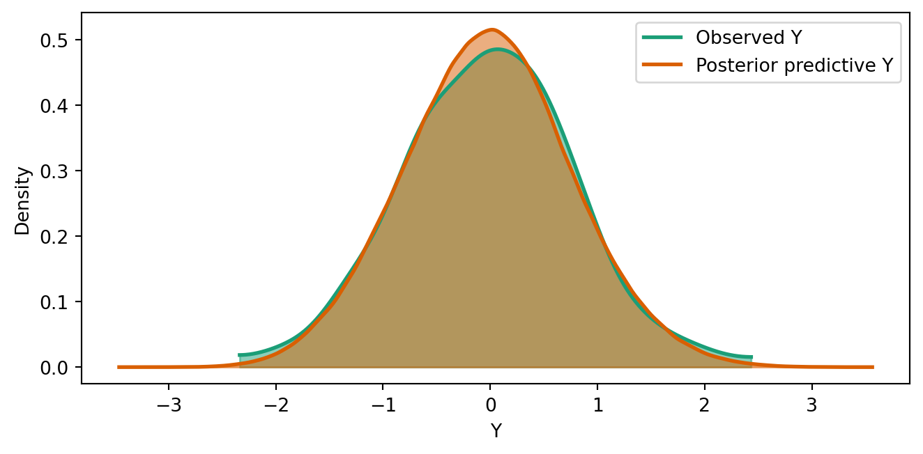

(a) Posterior predictive check: distribution of predicted Y values (orange) vs observed Y values (green).

(b)

(c)

Figure 4

7. Causal queries

With a well-checked model, causal queries carry full posterior uncertainty through the structural equations via g-computation.

model.ate("Y", "X", values=(0, 1))

ATE of X on Y

Mean	0.71
94% HDI	[0.68, 0.74]
P(> 0)	1.00
Draws	2000

Methods: .hdi() .prob() .summary() .draws() .by_time()

model.effect("X -> M -> Y")

EffectResult — X -> M -> Y

Mean	0.3791
SD	0.0245
94% HDI	[0.3349, 0.4264]
P(> 0)	1.0000
Draws	2000

Methods: .hdi()  ·  Attributes: .mean .sd .prob_gt_zero .draws

The ATE should be close to the true total effect (a \times b + c = 0.5 \times 0.8 + 0.3 = 0.7), and the indirect effect through M should be close to a \times b = 0.4.

Summary

Step	Method	Cost
Build model	pathmc.model(spec, data)	Instant
Inspect	graph(), equations()	Instant
Prior predictive check	sample_prior_predictive()	Seconds
Refine priors	set_priors()	Instant
Fit	fit()	Minutes
Posterior checks	summary(), effects_summary(), predict()	Seconds
Causal queries	ate(), do(), prob(), effect()	Seconds

The first four steps form a fast inner loop that you can repeat many times before committing to MCMC. The outer loop — revising the model specification itself — is for when posterior checks reveal structural problems.

Further reading

• Custom Priors — deeper dive into prior specification with hierarchical priors and different distribution families
• Model Specification — DSL syntax reference
• Causal Inference — the do-operator and g-computation
• Standardized Effects — comparing effect sizes across scales