Custom Priors
Refine prior distributions using an iterative inspect-check-refine workflow with prior predictive checks.
Every Bayesian model encodes assumptions about plausible parameter values before seeing data. pathmc ships with weakly informative defaults that work out of the box, but domain knowledge almost always lets you do better. Tighter, more realistic priors improve sampling efficiency, reduce the influence of prior-data conflict, and — critically for causal inference — produce more credible interventional predictions from do().
This example walks through the iterative prior workflow: inspect the defaults, run a prior predictive check, refine, and verify.
Simulate data with known structure
We generate data from a simple causal chain where a treatment X affects an outcome Y through a mediator M, with known coefficients.
import numpy as np
import pandas as pd
import pathmc
from pathmc import Prior

rng = np.random.default_rng(42)
n = 500

X = rng.normal(size=n)
M = 0.5 * X + rng.normal(scale=0.3, size=n)
Y = 0.8 * M + 0.3 * X + rng.normal(scale=0.3, size=n)

df = pd.DataFrame({"X": X, "M": M, "Y": Y})
True values: a = 0.5, b = 0.8, c = 0.3, \sigma_M = 0.3, \sigma_Y = 0.3.
Inspect the default priors
When you call pathmc.model() without specifying priors, sensible defaults are used. The .equations() method shows the structural equations alongside the priors.
spec = """
M ~ a*X
Y ~ b*M + c*X
"""

model = pathmc.model(spec, data=df)
model.equations()
\begin{aligned} \beta_{M} &\sim \text{Normal}(mu=0,\, sigma=10) \\ \sigma_{M} &\sim \text{HalfNormal}(sigma=1) \\ \beta_{Y} &\sim \text{Normal}(mu=0,\, sigma=10) \\ \sigma_{Y} &\sim \text{HalfNormal}(sigma=1) \\[6pt] \mu_{M} &= \beta_{0,\,M} + a \cdot \mathrm{X} \\ \mathrm{M} &\sim \text{Normal}(\mu_{M},\, \sigma_{M}) \\ \mu_{Y} &= \beta_{0,\,Y} + b \cdot \mathrm{M} + c \cdot \mathrm{X} \\ \mathrm{Y} &\sim \text{Normal}(\mu_{Y},\, \sigma_{Y}) \end{aligned}
The defaults are deliberately vague: Normal(mu=0, sigma=10) for regression coefficients and HalfNormal(sigma=1) for residual standard deviations. These are reasonable starting points when you know nothing about the scale of your data, but they may be wider than necessary.
Prior predictive check: are defaults plausible?
A prior predictive check asks: “If we sampled parameters from our priors and generated fake data, would it look remotely like real-world data?” If the prior implies outcomes spanning thousands of units when the real data lives in [-3, 3], the priors are too vague.
Code
import matplotlib.pyplot as plt
import arviz as az

FIG_WIDTH = 7
FIG_HEIGHT = 3.5

COLOR_DEFAULT = "#1b9e77"
COLOR_CUSTOM = "#d95f02"
COLOR_TRUE = "black"
ppc_default = model.sample_prior_predictive(draws=500, random_seed=42)Sampling: [M, Y, beta_M, beta_Y, sigma_M, sigma_Y]Code
y_prior = ppc_default.prior["Y"].values.flatten()

fig, ax = plt.subplots(figsize=(FIG_WIDTH, FIG_HEIGHT))
x_kde, y_kde, _ = az.kde(y_prior)
ax.plot(x_kde, y_kde, color=COLOR_DEFAULT, lw=2, label="Prior predictive (default)")
ax.fill_between(x_kde, y_kde, alpha=0.6, color=COLOR_DEFAULT)
ax.axvline(
    df["Y"].mean(),
    color=COLOR_TRUE,
    linestyle="--",
    linewidth=1.5,
    label=f"Observed mean = {df['Y'].mean():.2f}",
)
ax.set_xlabel("Y")
ax.set_ylabel("Density")
ax.legend()
ax.set_title("Prior predictive: default priors")
plt.tight_layout()
plt.show()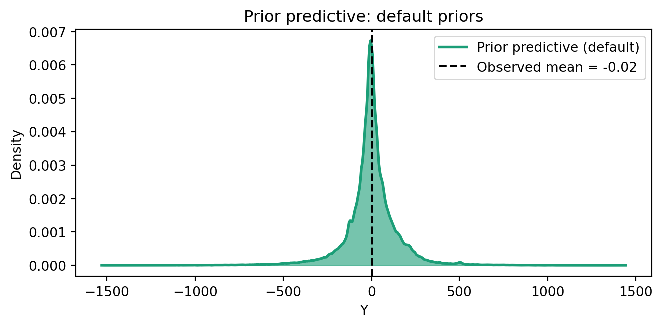
The default priors generate Y values spanning a huge range. For this dataset, where Y lives roughly in [-2, 2], coefficients of \pm 10 are implausible. We can do better.
Refine priors with set_priors()
The set_priors() method lets you override specific priors without re-specifying the model. It merges your changes with the current configuration and recompiles.
Since we know the predictors and outcomes are roughly standard-normal, regression coefficients above \pm 3 in magnitude are implausible. We also know the residual noise should be moderate — not zero, but not 10 either.
model.set_priors({
    "beta_M": Prior("Normal", mu=0, sigma=2),
    "beta_Y": Prior("Normal", mu=0, sigma=2),
    "sigma_M": Prior("HalfNormal", sigma=0.5),
    "sigma_Y": Prior("HalfNormal", sigma=0.5),
})

model.equations()
\begin{aligned} \beta_{M} &\sim \text{Normal}(mu=0,\, sigma=2) \\ \sigma_{M} &\sim \text{HalfNormal}(sigma=0.5) \\ \beta_{Y} &\sim \text{Normal}(mu=0,\, sigma=2) \\ \sigma_{Y} &\sim \text{HalfNormal}(sigma=0.5) \\[6pt] \mu_{M} &= \beta_{0,\,M} + a \cdot \mathrm{X} \\ \mathrm{M} &\sim \text{Normal}(\mu_{M},\, \sigma_{M}) \\ \mu_{Y} &= \beta_{0,\,Y} + b \cdot \mathrm{M} + c \cdot \mathrm{X} \\ \mathrm{Y} &\sim \text{Normal}(\mu_{Y},\, \sigma_{Y}) \end{aligned}
ppc_custom = model.sample_prior_predictive(draws=500, random_seed=42)Sampling: [M, Y, beta_M, beta_Y, sigma_M, sigma_Y]Code
y_default = ppc_default.prior["Y"].values.flatten()
y_custom = ppc_custom.prior["Y"].values.flatten()

fig, ax = plt.subplots(figsize=(FIG_WIDTH, FIG_HEIGHT))

x_kde, y_kde, _ = az.kde(y_default)
ax.plot(x_kde, y_kde, color=COLOR_DEFAULT, lw=2, label="Default priors")
ax.fill_between(x_kde, y_kde, alpha=0.45, color=COLOR_DEFAULT)
x_kde, y_kde, _ = az.kde(y_custom)
ax.plot(x_kde, y_kde, color=COLOR_CUSTOM, lw=2, label="Custom priors")
ax.fill_between(x_kde, y_kde, alpha=0.55, color=COLOR_CUSTOM)
ax.axvline(
    df["Y"].mean(),
    color=COLOR_TRUE,
    linestyle="--",
    linewidth=1.5,
    label=f"Observed mean = {df['Y'].mean():.2f}",
)
ax.set_xlabel("Y")
ax.set_ylabel("Density")
ax.legend()
ax.set_title("Prior predictive comparison")
plt.tight_layout()
plt.show()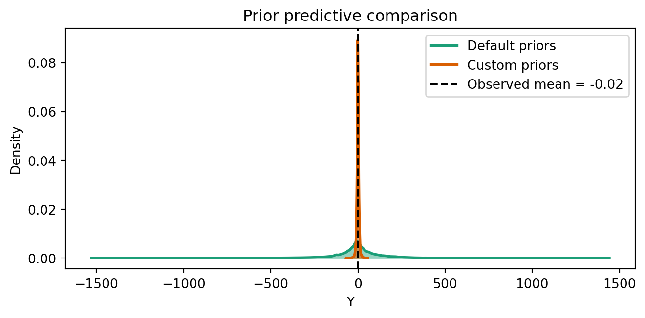
The custom priors concentrate probability mass in the plausible range. The model still allows coefficients up to \pm 4–6 (the 2\sigma range of Normal(0, 2)), which is generous, but it no longer considers coefficients of 10 or 20 as likely.
Sample and verify
With priors that encode our domain knowledge, we can proceed to posterior inference.
model.fit(draws=500, tune=500, chains=4, random_seed=42)NUTS[nutpie]: [beta_Y, sigma_M, beta_M, sigma_Y]<xarray.DataTree>
Group: /
├── Group: /posterior
│ Dimensions: (chain: 4, draw: 500, Y_predictors: 3, M_predictors: 2,
│ mu_Y_dim_0: 500, mu_M_dim_0: 500)
│ Coordinates:
│ * chain (chain) int64 32B 0 1 2 3
│ * draw (draw) int64 4kB 0 1 2 3 4 5 6 ... 493 494 495 496 497 498 499
│ * Y_predictors (Y_predictors) object 24B 'Intercept' 'M' 'X'
│ * M_predictors (M_predictors) object 16B 'Intercept' 'X'
│ * mu_Y_dim_0 (mu_Y_dim_0) int64 4kB 0 1 2 3 4 5 ... 494 495 496 497 498 499
│ * mu_M_dim_0 (mu_M_dim_0) int64 4kB 0 1 2 3 4 5 ... 494 495 496 497 498 499
│ Data variables:
│ beta_Y (chain, draw, Y_predictors) float64 48kB 0.01076 ... 0.3407
│ beta_M (chain, draw, M_predictors) float64 32kB -0.01287 ... 0.5213
│ sigma_M (chain, draw) float64 16kB 0.2867 0.3084 ... 0.2913 0.3228
│ sigma_Y (chain, draw) float64 16kB 0.297 0.3052 ... 0.3113 0.3007
│ mu_Y (chain, draw, mu_Y_dim_0) float64 8MB 0.5402 ... -0.8795
│ mu_M (chain, draw, mu_M_dim_0) float64 8MB 0.1378 ... -0.7864
│ Attributes:
│ created_at: 2026-07-31T15:49:08.431186+00:00
│ creation_library: ArviZ
│ creation_library_version: 1.1.0
│ creation_library_language: Python
│ sample_dims: ['chain', 'draw']
│ inference_library: nutpie
│ inference_library_version: 0.16.10
│ sampling_time: 0.10288691520690918
│ tuning_steps: 500
├── Group: /sample_stats
│ Dimensions: (chain: 4, draw: 500)
│ Coordinates:
│ * chain (chain) int64 32B 0 1 2 3
│ * draw (draw) int64 4kB 0 1 2 3 4 ... 495 496 497 498 499
│ Data variables: (12/20)
│ depth (chain, draw) uint64 16kB 2 3 3 2 2 ... 2 2 3 3 3
│ maxdepth_reached (chain, draw) bool 2kB False False ... False False
│ step_size (chain, draw) float64 16kB 0.6706 0.652 ... 0.7469
│ transformation_update_id (chain, draw) int64 16kB 0 0 0 0 0 0 ... 0 0 0 0 0
│ step_size_bar (chain, draw) float64 16kB 0.7114 ... 0.7294
│ mean_tree_accept (chain, draw) float64 16kB 0.5497 ... 0.9232
│ ... ...
│ fisher_distance (chain, draw) float64 16kB 0.1828 0.2064 ... 0.304
│ transformation_index (chain, draw) int64 16kB 420 420 420 ... 423 423
│ diverging (chain, draw) bool 2kB False False ... False False
│ divergence_draw (chain, draw) uint64 16kB 0 0 0 0 0 ... 0 0 0 0 0
│ divergence_message (chain, draw) object 16kB None None ... None None
│ divergence_energy_error (chain, draw) float64 16kB nan nan nan ... nan nan
│ Attributes:
│ created_at: 2026-07-31T15:49:08.425129+00:00
│ creation_library: ArviZ
│ creation_library_version: 1.1.0
│ creation_library_language: Python
│ sample_dims: ['chain', 'draw']
│ inference_library: nutpie
│ inference_library_version: 0.16.10
│ inference_library_settings: {"sampler": "nuts", "adaptation": "diag", "s...
├── Group: /constant_data
│ Dimensions: (X_dim_0: 500)
│ Coordinates:
│ * X_dim_0 (X_dim_0) int64 4kB 0 1 2 3 4 5 6 7 ... 493 494 495 496 497 498 499
│ Data variables:
│ X (X_dim_0) float64 4kB 0.3047 -1.04 0.7505 ... -0.3356 -1.991 -1.495
│ Attributes:
│ created_at: 2026-07-31T15:49:08.428361+00:00
│ creation_library: ArviZ
│ creation_library_version: 1.1.0
│ creation_library_language: Python
│ inference_library: pymc
│ inference_library_version: 6.0.1
│ sample_dims: []
├── Group: /observed_data
│ Dimensions: (M_dim_0: 500, Y_dim_0: 500)
│ Coordinates:
│ * M_dim_0 (M_dim_0) int64 4kB 0 1 2 3 4 5 6 7 ... 493 494 495 496 497 498 499
│ * Y_dim_0 (Y_dim_0) int64 4kB 0 1 2 3 4 5 6 7 ... 493 494 495 496 497 498 499
│ Data variables:
│ M (M_dim_0) float64 4kB 0.5615 -0.2514 0.1594 ... -0.9562 -0.5004
│ Y (Y_dim_0) float64 4kB 0.5228 -0.7319 0.2283 ... -1.149 -1.203
│ Attributes:
│ created_at: 2026-07-31T15:49:08.430033+00:00
│ creation_library: ArviZ
│ creation_library_version: 1.1.0
│ creation_library_language: Python
│ inference_library: pymc
│ inference_library_version: 6.0.1
│ sample_dims: []
└── Group: /log_likelihood
Dimensions: (chain: 4, draw: 500, M_dim_0: 500, Y_dim_0: 500)
Coordinates:
* chain (chain) int64 32B 0 1 2 3
* draw (draw) int64 4kB 0 1 2 3 4 5 6 7 ... 493 494 495 496 497 498 499
* M_dim_0 (M_dim_0) int64 4kB 0 1 2 3 4 5 6 7 ... 493 494 495 496 497 498 499
* Y_dim_0 (Y_dim_0) int64 4kB 0 1 2 3 4 5 6 7 ... 493 494 495 496 497 498 499
Data variables:
M (chain, draw, M_dim_0) float64 8MB -0.7618 -0.1313 ... -0.1807
Y (chain, draw, Y_dim_0) float64 8MB 0.2933 0.05542 ... -0.2971
Attributes:
created_at: 2026-07-31T15:49:08.522062+00:00
creation_library: ArviZ
creation_library_version: 1.1.0
creation_library_language: Python
inference_library: pymc
inference_library_version: 6.0.1
sample_dims: ['chain', 'draw']model.effects_summary()| mean | sd | hdi_3% | hdi_97% | |
|---|---|---|---|---|
| name | ||||
| a | 0.496857 | 0.014193 | 0.469224 | 0.523093 |
| b | 0.763104 | 0.044793 | 0.680660 | 0.847168 |
| c | 0.334709 | 0.026554 | 0.288000 | 0.386576 |
The posterior means should be close to the true values (a = 0.5, b = 0.8, c = 0.3).
Specifying priors up front
If you already know your priors before fitting, you can pass them directly to model() instead of using the two-step inspect-then-refine approach.
model_upfront = pathmc.model(
    spec,
    data=df,
    priors={
        "beta_M": Prior("Normal", mu=0, sigma=2),
        "beta_Y": Prior("Normal", mu=0, sigma=2),
        "sigma_M": Prior("HalfNormal", sigma=0.5),
        "sigma_Y": Prior("HalfNormal", sigma=0.5),
    },
)

model_upfront.equations()
\begin{aligned} \beta_{M} &\sim \text{Normal}(mu=0,\, sigma=2) \\ \sigma_{M} &\sim \text{HalfNormal}(sigma=0.5) \\ \beta_{Y} &\sim \text{Normal}(mu=0,\, sigma=2) \\ \sigma_{Y} &\sim \text{HalfNormal}(sigma=0.5) \\[6pt] \mu_{M} &= \beta_{0,\,M} + a \cdot \mathrm{X} \\ \mathrm{M} &\sim \text{Normal}(\mu_{M},\, \sigma_{M}) \\ \mu_{Y} &= \beta_{0,\,Y} + b \cdot \mathrm{M} + c \cdot \mathrm{X} \\ \mathrm{Y} &\sim \text{Normal}(\mu_{Y},\, \sigma_{Y}) \end{aligned}
Both approaches produce the same compiled model.
Using different distribution families
The Prior class supports any PyMC distribution. When domain knowledge suggests a specific shape — for example, that a coefficient should be positive, or bounded — you can express that directly.
model_informative = pathmc.model(
    spec,
    data=df,
    priors={
        "sigma_M": Prior("Exponential", lam=3),
        "sigma_Y": Prior("Exponential", lam=3),
    },
)

model_informative.equations()
\begin{aligned} \beta_{M} &\sim \text{Normal}(mu=0,\, sigma=10) \\ \sigma_{M} &\sim \text{Exponential}(lam=3) \\ \beta_{Y} &\sim \text{Normal}(mu=0,\, sigma=10) \\ \sigma_{Y} &\sim \text{Exponential}(lam=3) \\[6pt] \mu_{M} &= \beta_{0,\,M} + a \cdot \mathrm{X} \\ \mathrm{M} &\sim \text{Normal}(\mu_{M},\, \sigma_{M}) \\ \mu_{Y} &= \beta_{0,\,Y} + b \cdot \mathrm{M} + c \cdot \mathrm{X} \\ \mathrm{Y} &\sim \text{Normal}(\mu_{Y},\, \sigma_{Y}) \end{aligned}
TipDiscovering valid prior keys
Call .equations() on any model to see both the structural equations and the full list of prior parameter names you can customize. Use .equations(show="priors") to see only the priors. The keys depend on your model specification — a model with random slopes will have mu_slope_* and sigma_slope_* keys, while a model with transforms will include the transform parameter names.
Summary
- Default priors (
Normal(0, 10)for coefficients,HalfNormal(1)for scales) work out of the box and require zero configuration. .equations()shows the structural equations and the current prior specification for every model parameter. Useshow="priors"to see only the priors..sample_prior_predictive()generates data from the prior to verify that your assumptions produce plausible outcomes..set_priors()merges overrides into the current prior configuration and recompiles the model. Only the specified parameters change; everything else keeps its current value.model(priors=...)accepts priors at creation time for a one-step workflow.- Any PyMC distribution can serve as a prior via
Prior("DistName", ...)frompymc_extras. - The iterative workflow — inspect, check, refine, re-check, sample — is the principled approach to prior specification in Bayesian modeling. See Bayesian Workflow for the full end-to-end cycle from model specification through causal queries.
NoteAdapt this to your domain
Consider the quantities in your own causal model. What range of coefficient values would be scientifically absurd? If a 1-unit change in an input could never plausibly produce a 50-unit change in the outcome, a Normal(0, 10) prior is too generous.
- Clinical trials: effect sizes above 1–2 standard deviations are rare; a
Normal(0, 1)orNormal(0, 2)on standardized coefficients is often appropriate. - Marketing: elasticities (percent change in sales per percent change in spend) are typically in [0, 0.5]; a
HalfNormal(sigma=0.3)keeps the prior realistic. - Economics: use prior studies or meta-analyses to set informative priors on known structural parameters.