Nonparametric Smooths with HSGP

Fit a flexible 1-D nonparametric smooth with the hsgp() term — a Hilbert Space Gaussian Process approximation — and intervene on it with do().

Author

PyMC Labs

Most pathmc terms are linear in their coefficients. Sometimes the relationship between a predictor and an outcome is smooth but not linear — a dose–response curve, a trend over a continuous index, a smooth confounder adjustment. The hsgp() term adds such a smooth via a Hilbert Space Gaussian Process approximation (riutort2023practical?), the same scalable construction exposed by Bambi’s hsgp().

An HSGP approximates a Gaussian process with a finite basis of Laplacian eigenfunctions, so it reduces to a linear model in a fixed basis matrix. That makes it fast, differentiable, and — because the basis is a deterministic function of the input pm.Data — fully compatible with do() interventions.

Simulated data

We draw a smooth signal and add observation noise. The input is deliberately not centered on zero to exercise the internal centering of the basis.

import numpy as np
import pandas as pd

import pathmc

rng = np.random.default_rng(0)
x = np.linspace(10.0, 20.0, 120)
true = np.sin((x - 10.0) * 0.9)
y = true + rng.normal(0.0, 0.2, size=x.size)
df = pd.DataFrame({"x": x, "y": y})

The model

hsgp(x, m=..., c=...) is a standalone term: m sets the number of basis vectors and c the boundary-expansion factor. The smooth carries its own basis weights, so it takes no coefficient prefix.

model = pathmc.model("y ~ hsgp(x, m=20, c=1.5)", data=df)
model.equations()

\begin{aligned} \beta_{y} &\sim \text{Normal}(mu=0,\, sigma=10) \\ \sigma_{y} &\sim \text{HalfNormal}(sigma=1) \\ \ell_{y,x} &\sim \text{InverseGamma}(alpha=3,\, beta=1) \\ \eta_{y,x} &\sim \text{HalfNormal}(sigma=1) \\ \beta_{hsgp,y,x} &\sim \text{Normal}(mu=0,\, sigma=1) \\[6pt] \mu_{y} &= \beta_{0,\,y} + f_{\mathrm{hsgp}}(\mathrm{x}) \\ \mathrm{y} &\sim \text{Normal}(\mu_{y},\, \sigma_{y}) \end{aligned}

The default priors expose the kernel amplitude (eta_y_x), lengthscale (ell_y_x), and standardized basis weights (beta_hsgp_y_x):

model.priors()

The lengthscale prior is in raw input units: the default InverseGamma(3, 1) has mean 0.5, so an input spanning a wide range pulls against it and can produce divergences — standardize the input, override ell_y_x, or raise target_accept as we do below. A range-scaled default is tracked in issue #375.

Fit and recover the smooth

idata = model.fit(random_seed=0, target_accept=0.99)
f_mean = idata.posterior["f_y_x"].mean(("chain", "draw")).values
np.corrcoef(f_mean - f_mean.mean(), true - true.mean())[0, 1]

NUTS[nutpie]: [eta_y_x, ell_y_x, beta_hsgp_y_x, beta_y, sigma_y]

np.float64(0.9968956933462689)

The posterior-mean smooth tracks the true function closely. To show that honestly we plot the posterior of mu_y — the full linear predictor, which already carries the intercept — as a mean line with a 94% highest-density interval, rather than recentering f_y_x by hand.

Code

import arviz as az
import matplotlib.pyplot as plt

mu = idata.posterior["mu_y"]
mu_mean = mu.mean(("chain", "draw")).values
hdi = az.hdi(mu, prob=0.94).values

fig, ax = plt.subplots(figsize=(8, 4))
ax.scatter(x, y, s=12, alpha=0.5, color="C0", label="observed")
ax.fill_between(x, hdi[:, 0], hdi[:, 1], color="C1", alpha=0.3, label="94% HDI")
ax.plot(x, mu_mean, "C1", lw=2, label="posterior mean")
ax.plot(x, true, "k--", lw=1.5, label="true smooth")
ax.set(xlabel="x", ylabel="y")
ax.legend()
plt.show()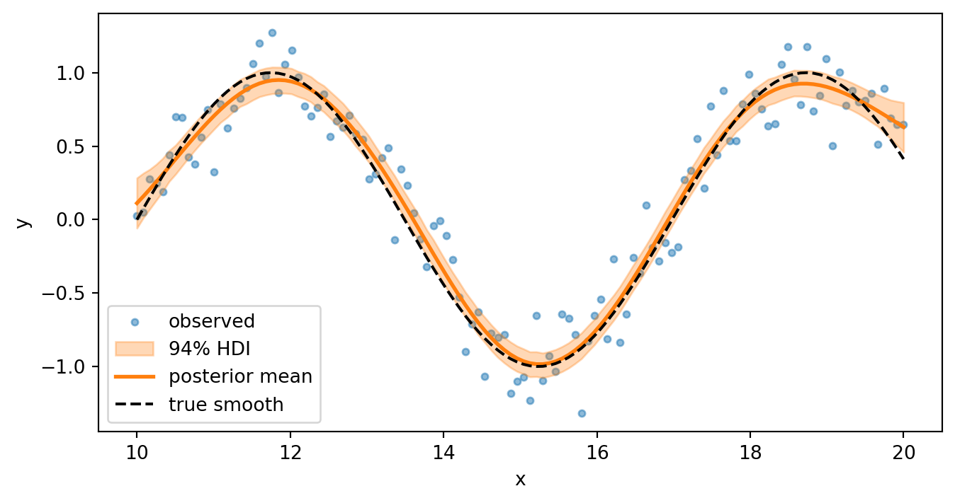

Figure 1: Posterior mean of mu_y with its 94% HDI, against the true smooth. The band covers the true curve across the fitted range of x, and widens at the boundaries where the basis is least constrained by data.

Intervening on the smooth

Because the basis recomputes from the input data node, do() propagates through the smooth. Interventions must stay within the basis boundary [mid − L, mid + L] frozen from the fitted data — with c > 1 this is wider than the data range, so moderate extrapolation is fine. Beyond the boundary the sinusoidal eigenfunctions alias rather than extrapolate, so do() raises a ValueError there instead of returning a plausible-looking but meaningless number.

low = model.do(set={"x": 12.0}).mean("y")
high = model.do(set={"x": 18.0}).mean("y")
low, high

(0.9417490558663085, 0.7755178003188019)

Scope

Phase 1 supports a single 1-D exogenous input on cross-sectional models. Multi-dimensional inputs, grouped (by=) GPs, and panel/scan models raise a clear error and are tracked as follow-ups.

The input must be exogenous because the basis is built by evaluating it: PyMC derives the centering midpoint and the boundary from the input’s realized values. Smoothing an endogenous variable (one that is itself the outcome of another equation) would freeze the basis at a random prior draw, so pathmc rejects it rather than fitting a model whose result depends on compilation-time RNG.