Mediation Analysis

Estimate direct and indirect effects through mediators — from a single pathway to correlated parallel mediators and latent variables with sparse measurements.

Author

Benjamin Vincent

A flat regression of treatment on outcome gives you the total effect — but says nothing about why the treatment works. Mediation analysis decomposes the total effect into the pathway that passes through an intermediate variable (the indirect effect) and the remainder (the direct effect).

This notebook builds mediation models of increasing complexity:

Classic mediation — a single mediator with labeled coefficients and defined parameters
Parallel mediators with correlated residuals — multiple pathways plus the ~~ operator for unmodeled common causes
Latent mediator with sparse measurements — a mediator that is mostly unobserved, anchored by a handful of noisy observations

Each section fits a model to simulated data with known true values, so we can verify that pathmc recovers the target quantities.

1. Classic mediation

The causal structure

A treatment X causes a mediator M, which in turn causes the outcome Y. X may also affect Y directly.

Figure 1: Classic mediation DAG. X affects Y directly (c) and indirectly through M (a × b).

The indirect effect is the product a \times b, and the total effect is c + a \times b.

Simulate data

import numpy as np
import pandas as pd
import matplotlib.pyplot as plt
import arviz as az
import pymc as pm
import pathmc

FIG_WIDTH = 7
FIG_HEIGHT = 3

rng = np.random.default_rng(42)
n = 500

X = rng.normal(size=n)
M = 0.5 * X + rng.normal(scale=0.5, size=n)
Y = 0.8 * M + 0.3 * X + rng.normal(scale=0.5, size=n)

df = pd.DataFrame({"X": X, "M": M, "Y": Y})
df.head()

	X	M	Y
0	0.304717	0.834290	0.729206
1	-1.039984	-0.072400	-0.734558
2	0.750451	0.015485	0.030287
3	0.940565	-0.280969	0.374349
4	-1.951035	-2.457782	-2.550040

True values: a = 0.5, b = 0.8, c = 0.3, indirect = 0.4, total = 0.7.

Specify and fit the model

The spec uses labeled coefficients (a*X, b*M, c*X) and defined parameters (:=) for derived quantities. Labels attach names to regression weights; defined parameters compute arbitrary posterior-draw-level expressions from those labels.

spec = """
M ~ a*X
Y ~ b*M + c*X
indirect := a*b
total := c + a*b
"""

model = pathmc.model(spec, data=df)

model.graph()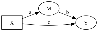

model.equations()

\begin{aligned} \beta_{M} &\sim \text{Normal}(mu=0,\, sigma=10) \\ \sigma_{M} &\sim \text{HalfNormal}(sigma=1) \\ \beta_{Y} &\sim \text{Normal}(mu=0,\, sigma=10) \\ \sigma_{Y} &\sim \text{HalfNormal}(sigma=1) \\[6pt] \mu_{M} &= \beta_{0,\,M} + a \cdot \mathrm{X} \\ \mathrm{M} &\sim \text{Normal}(\mu_{M},\, \sigma_{M}) \\ \mu_{Y} &= \beta_{0,\,Y} + b \cdot \mathrm{M} + c \cdot \mathrm{X} \\ \mathrm{Y} &\sim \text{Normal}(\mu_{Y},\, \sigma_{Y}) \\ indirect &\equiv a \cdot b \\ total &\equiv c + a \cdot b \end{aligned}

model.fit(draws=500, tune=500, chains=4, random_seed=42)

NUTS[nutpie]: [beta_Y, sigma_M, beta_M, sigma_Y]

Effects summary

effects_summary() focuses on labeled coefficients and defined parameters — the quantities with direct causal interpretation:

model.effects_summary()

	mean	sd	hdi_3%	hdi_97%
name
a	0.496374	0.024385	0.451510	0.544045
b	0.762303	0.043422	0.675802	0.836618
c	0.346322	0.032509	0.287843	0.410019
indirect	0.378394	0.028626	0.323829	0.430932
total	0.724716	0.030751	0.672427	0.788413

The indirect row shows the posterior distribution of a \times b, computed element-wise over posterior draws.

Path-specific effects

The effect() method computes path-specific effects by multiplying coefficient draws along a specified path:

indirect = model.effect("X -> M -> Y")
indirect

EffectResult — X -> M -> Y

Mean	0.3784
SD	0.0286
94% HDI	[0.3238, 0.4309]
P(> 0)	1.0000
Draws	2000

Methods: .hdi() · Attributes: .mean .sd .prob_gt_zero .draws

direct = model.effect("X -> Y")
direct

EffectResult — X -> Y

Mean	0.3463
SD	0.0325
94% HDI	[0.2878, 0.4100]
P(> 0)	1.0000
Draws	2000

Methods: .hdi() · Attributes: .mean .sd .prob_gt_zero .draws

Causal effect via do()

The total causal effect of X on Y flows through both the direct and indirect paths. We can verify this with do():

ate = model.ate("Y", "X", values=(0.0, 1.0))
ate

ATE of X on Y

Mean	0.72
94% HDI	[0.67, 0.79]
P(> 0)	1.00
Draws	2000

Methods: .hdi() .prob() .summary() .draws() .by_time() .dataset

The total effect should be close to the true value of 0.7 (direct 0.3 + indirect 0.4 via M). Fixing the mediator blocks the indirect path, isolating the direct effect:

r_d0 = model.do(set={"X": 0.0, "M": 0.0})
r_d1 = model.do(set={"X": 1.0, "M": 0.0})
direct_only = r_d1 - r_d0
direct_only

DoResult — 2000 draws, 3 variables

variable	mean	94% HDI
X	1.00	[1.00, 1.00]
M	0.00	[0.00, 0.00]
Y	0.35	[0.29, 0.41]

Methods: .draws() .mean() .hdi() .by_time() .dataset

The direct-only estimate should be close to 0.3 — the true direct effect, with the mediated path held fixed.

Standardized effects

When predictors are measured on different scales, raw coefficients are not directly comparable. .standardized() computes stdyx-standardized coefficients — the expected SD change in the outcome per SD change in the predictor:

model.standardized()

	predictor	outcome	mean	sd	hdi_3%	hdi_97%
name
a	X	M	0.683942	0.033599	0.622126	0.749627
b	M	Y	0.561879	0.032006	0.498121	0.616656
c	X	Y	0.351728	0.033016	0.292335	0.416419

Sequential ignorability

The direct/indirect decomposition requires a strong assumption beyond “no unmeasured confounders” for the total effect: there must be no unmeasured common cause of M and Y.

If an omitted variable drives both the mediator and the outcome, the coefficients b and c absorb its influence — the indirect and direct effects are biased even when the total effect is identified. This assumption, called sequential ignorability (Imai et al., 2010), is untestable from data alone.

In this example the DGP satisfies it by construction, but in real applications you should ask: “could anything cause both M and Y that I haven’t measured?”

The classic model handles one mediator cleanly. But what if a treatment operates through multiple mediators that share an unobserved common cause?

2. Parallel mediators with correlated residuals

The causal structure

A treatment T affects an outcome Y through two parallel mediators M1 and M2. The mediators share an unobserved common cause — for instance, an unmeasured personality trait that influences both learning styles. Ignoring this correlation biases the individual indirect effects.

The ~~ operator in pathmc accounts for this by fitting a multivariate normal block with an LKJ prior on the residual correlation matrix.

Figure 2: Parallel mediators DAG. T affects Y through M1 and M2. The dashed bidirected edge represents residual correlation from an unmodeled common cause.

Simulate data

The correlated residuals are generated from a bivariate normal with known covariance.

rng2 = np.random.default_rng(42)
n2 = 500

T = rng2.normal(size=n2)

eps = rng2.multivariate_normal(
    [0, 0],
    [[0.16, 0.08], [0.08, 0.16]],
    size=n2,
)

M1 = 0.6 * T + eps[:, 0]
M2 = 0.4 * T + eps[:, 1]
Y2 = 0.5 * M1 + 0.3 * M2 + 0.2 * T + rng2.normal(scale=0.5, size=n2)

df2 = pd.DataFrame({"T": T, "M1": M1, "M2": M2, "Y": Y2})

True values: a_1 = 0.6, a_2 = 0.4, b_1 = 0.5, b_2 = 0.3, c = 0.2. True residual correlation between M1 and M2 is 0.08 / 0.16 = 0.5.

Specify the model

The ~~ line declares the residual covariance block. Defined parameters capture both indirect effects and the total effect.

spec2 = """
M1 ~ a1*T
M2 ~ a2*T
Y  ~ b1*M1 + b2*M2 + c*T

M1 ~~ M2

indirect1 := a1*b1
indirect2 := a2*b2
total     := c + a1*b1 + a2*b2
"""

model2 = pathmc.model(spec2, data=df2)
model2.equations()

\begin{aligned} \beta_{M1} &\sim \text{Normal}(mu=0,\, sigma=10) \\ \sigma_{M1} &\sim \text{HalfNormal}(sigma=1) \\ \beta_{M2} &\sim \text{Normal}(mu=0,\, sigma=10) \\ \sigma_{M2} &\sim \text{HalfNormal}(sigma=1) \\ \beta_{Y} &\sim \text{Normal}(mu=0,\, sigma=10) \\ \sigma_{Y} &\sim \text{HalfNormal}(sigma=1) \\ chol_{M1,M2} &\sim \text{LKJCholeskyCov}(eta=2,\, sd\_dist=HalfNormal(1)) \\[6pt] \mu_{M1} &= \beta_{0,\,M1} + a1 \cdot \mathrm{T} \\ \mathrm{M1} &\sim \text{Normal}(\mu_{M1},\, \sigma_{M1}) \\ \mu_{M2} &= \beta_{0,\,M2} + a2 \cdot \mathrm{T} \\ \mathrm{M2} &\sim \text{Normal}(\mu_{M2},\, \sigma_{M2}) \\ \mu_{Y} &= \beta_{0,\,Y} \\ &\quad + b1 \cdot \mathrm{M1} \\ &\quad + b2 \cdot \mathrm{M2} \\ &\quad + c \cdot \mathrm{T} \\ \mathrm{Y} &\sim \text{Normal}(\mu_{Y},\, \sigma_{Y}) \\ indirect1 &\equiv a1 \cdot b1 \\ indirect2 &\equiv a2 \cdot b2 \\ total &\equiv c + a1 \cdot b1 + a2 \cdot b2 \end{aligned}

model2.graph()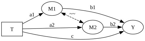

model2.fit(draws=500, tune=500, chains=4, random_seed=42)

NUTS[nutpie]: [beta_Y, beta_M2, beta_M1, chol_M1_M2, sigma_Y]

Results

model2.effects_summary()

	mean	sd	hdi_3%	hdi_97%
name
a1	0.591218	0.020987	0.552347	0.629548
a2	0.391498	0.018815	0.355916	0.425599
b1	-0.101289	8.639138	-16.562781	15.653436
b2	0.208667	9.464869	-16.249769	18.564670
c	0.570768	5.687424	-9.540955	12.324438
indirect1	-0.065665	5.109775	-9.928073	9.060784
indirect2	0.082251	3.708612	-6.310876	7.360001
total	0.587354	0.025639	0.541150	0.635665

The summary includes the LKJ correlation parameter for the M1 ~~ M2 block alongside the regression coefficients.

Comparing indirect pathways

ind1 = model2.effect("T -> M1 -> Y")
ind2 = model2.effect("T -> M2 -> Y")

print(f"Indirect via M1: {ind1.mean:.3f}  (true: 0.300)")
print(f"Indirect via M2: {ind2.mean:.3f}  (true: 0.120)")

Indirect via M1: -0.066  (true: 0.300)
Indirect via M2: 0.082  (true: 0.120)

When to use ~~

The ~~ operator is appropriate when you believe two variables share an unmodeled common cause but cannot (or do not need to) measure it directly. It does not model a causal relationship between the two variables — it accounts for the correlation their residuals would exhibit due to the omitted cause.

If the common cause is measurable, including it as an explicit variable in the DAG is preferable because it makes the causal structure transparent and enables richer interventional queries.

We can now decompose a total effect through two correlated mediators. But what if the mediator itself is unobserved for most units?

3. Latent mediator with sparse measurements

The scenario

A company runs a training program and wants to know its causal effect on employee productivity. They suspect training works primarily by building skill — but skill is never directly measured for most employees. A small subset took a skills assessment, providing sparse, noisy anchor points.

The question: can we recover the causal pathway when the mediator is mostly unobserved?

The causal structure

Training (X) builds skill (M), which drives productivity (Y). Training may also affect productivity directly (e.g. through motivation), captured by coefficient c. A skills assessment (M_obs) provides a noisy measurement of skill for a subset of employees.

Figure 3: Training (X) builds latent skill (M, dashed border), which drives productivity (Y). Sparse skills assessments (M_obs) anchor the latent scale.

Component	Formula	Role
Structural	M \equiv a \cdot X	Deterministic latent — no noise, no data column
Outcome	Y = b \cdot M + c \cdot X + \varepsilon	Observed productivity
Measurement	M_\text{obs} = M + \eta	Sparse, noisy skills assessment

Simulate data

rng3 = np.random.default_rng(42)
n3 = 500

X3 = rng3.normal(size=n3)
M_true = 0.6 * X3 + rng3.normal(scale=0.4, size=n3)
Y3 = 0.7 * M_true + 0.2 * X3 + rng3.normal(scale=0.5, size=n3)

M_obs = np.full(n3, np.nan)
assessed = rng3.choice(n3, size=int(0.3 * n3), replace=False)
M_obs[assessed] = M_true[assessed] + rng3.normal(scale=0.3, size=len(assessed))

df3 = pd.DataFrame({"X": X3, "Y": Y3, "M_obs": M_obs})
print(f"Employees assessed: {(~np.isnan(M_obs)).sum()}/{n3}")

Employees assessed: 150/500

True values: a = 0.6, b = 0.7, c = 0.2, indirect = 0.42, total = 0.62.

Code

COLOR_ASSESSED = "#e07a2f"
COLOR_UNASSESSED = "#bbbbbb"
COLOR_ALL = "#4878cf"

fig, axes = plt.subplots(1, 2, figsize=(FIG_WIDTH, FIG_HEIGHT))

axes[0].scatter(X3, Y3, s=8, alpha=0.4, color=COLOR_ALL)
axes[0].set_xlabel("Training (X)")
axes[0].set_ylabel("Productivity (Y)")
axes[0].set_title("Observable data")

mask = ~np.isnan(M_obs)
axes[1].scatter(
    X3[~mask],
    M_true[~mask],
    s=8,
    alpha=0.25,
    color=COLOR_UNASSESSED,
    label="No assessment",
)
axes[1].scatter(
    X3[mask],
    M_true[mask],
    s=14,
    alpha=0.7,
    color=COLOR_ASSESSED,
    label="Assessed",
    zorder=3,
)
axes[1].set_xlabel("Training (X)")
axes[1].set_ylabel("True skill (M)")
axes[1].set_title("Latent skill — sparse assessment coverage")
axes[1].legend(fontsize=8, frameon=False)

plt.tight_layout()
plt.show()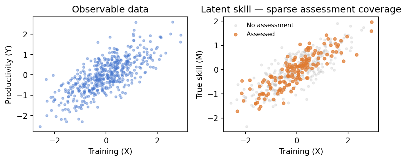

Figure 4: Left: training hours versus productivity for all 500 employees. Right: true latent skill versus training, highlighting the 30% with observed assessments (orange) versus unassessed employees (grey).

Specify and fit the model

Three features work together:

latent=["M"] tells pathmc that M has no observed data — it compiles as a deterministic node.
The measurement equation M_obs ~ 0 + 1*M connects the sparse assessment to the latent skill. Rows where M_obs is NaN contribute no measurement likelihood.
Defined parameters compute the indirect and total effects from posterior draws.

spec3 = """
M ~ a*X
Y ~ b*M + c*X
M_obs ~ 0 + 1*M
indirect := a*b
total := a*b + c
"""

model3 = pathmc.model(spec3, data=df3, latent=["M"])

/Users/benjamv/git/pathmc/.venv/lib/python3.12/site-packages/pymc/model/core.py:1337: ImputationWarning: Data in M_obs contains missing values and will be automatically imputed from the sampling distribution.
  warnings.warn(impute_message, ImputationWarning)

model3.equations()

\begin{aligned} \beta_{M} &\sim \text{Normal}(mu=0,\, sigma=10) \\ \beta_{Y} &\sim \text{Normal}(mu=0,\, sigma=10) \\ \sigma_{Y} &\sim \text{HalfNormal}(sigma=1) \\ \sigma_{M,obs} &\sim \text{HalfNormal}(sigma=1) \\[6pt] \mathrm{M} &\equiv \beta_{0,\,M} + a \cdot \mathrm{X} \\ \mu_{Y} &= \beta_{0,\,Y} + b \cdot \mathrm{M} + c \cdot \mathrm{X} \\ \mathrm{Y} &\sim \text{Normal}(\mu_{Y},\, \sigma_{Y}) \\ \mu_{M,obs} &= 1 \cdot \mathrm{M} \\ \mathrm{M\_obs} &\sim \text{Normal}(\mu_{M,obs},\, \sigma_{M,obs}) \\ indirect &\equiv a \cdot b \\ total &\equiv a \cdot b + c \end{aligned}

model3.graph()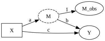

idata3 = model3.fit(draws=1000, tune=1000, chains=4, random_seed=42)

NUTS[nutpie]: [sigma_M_obs, beta_M, M_obs_unobserved, beta_Y, sigma_Y]

Effects summary

model3.effects_summary()

	mean	sd	hdi_3%	hdi_97%
name
a	0.613546	0.041113	0.537731	0.693742
b	0.645482	5.133045	-8.021678	9.858482
c	0.250933	3.150141	-5.672484	5.350066
indirect	0.393808	3.150787	-4.735443	6.303601
total	0.644741	0.026843	0.596398	0.695687

The coefficient a (training → skill) is tightly recovered thanks to the sparse assessments. The total effect concentrates near its true value of 0.62. But b and c individually have wide posteriors — the next figure explains why.

Identification: what’s anchored and what isn’t

The sparse measurements anchor the scale of the latent variable. Without them, the model cannot distinguish “large a, small b” from “small a, large b” — the product a \cdot b is all the data can constrain.

The remaining non-identifiability is between b and c. Because the latent M is a deterministic linear function of X (M \equiv \text{intercept} + a \cdot X), the predictors M and X are collinear in the outcome equation. The model can estimate b \cdot a + c precisely, but cannot separate b from c.

Code

COLOR_A = "#4878cf"
COLOR_BC = "#e07a2f"
COLOR_TOTAL = "#2ca02c"

fig, axes = plt.subplots(1, 3, figsize=(FIG_WIDTH, FIG_HEIGHT))

a_draws = idata3.posterior["beta_M"].sel(M_predictors="X").values.flatten()
x_kde, y_kde, _ = az.kde(a_draws)
axes[0].plot(x_kde, y_kde, color=COLOR_A, lw=2)
axes[0].fill_between(x_kde, y_kde, alpha=0.7, color=COLOR_A)
axes[0].axvline(0.6, color="black", ls="--", lw=1.2, label="True a = 0.6")
axes[0].set_xlabel("a (training → skill)")
axes[0].set_ylabel("Density")
axes[0].set_title("Well-identified")
axes[0].legend(fontsize=7, frameon=False)

b_draws = idata3.posterior["beta_Y"].sel(Y_predictors="M").values.flatten()
c_draws = idata3.posterior["beta_Y"].sel(Y_predictors="X").values.flatten()
x_kde, y_kde, _ = az.kde(b_draws)
axes[1].plot(x_kde, y_kde, color=COLOR_BC, lw=2, label="b (skill → prod.)")
axes[1].fill_between(x_kde, y_kde, alpha=0.4, color=COLOR_BC)
x_kde, y_kde, _ = az.kde(c_draws)
axes[1].plot(x_kde, y_kde, color=COLOR_BC, lw=2, label="c (direct)")
axes[1].fill_between(x_kde, y_kde, alpha=0.15, color=COLOR_BC)
axes[1].set_xlabel("Coefficient value")
axes[1].set_title("Not separately identified")
axes[1].legend(fontsize=7, frameon=False)

total_draws = a_draws * b_draws + c_draws
x_kde, y_kde, _ = az.kde(total_draws)
axes[2].plot(x_kde, y_kde, color=COLOR_TOTAL, lw=2)
axes[2].fill_between(x_kde, y_kde, alpha=0.7, color=COLOR_TOTAL)
axes[2].axvline(0.62, color="black", ls="--", lw=1.2, label="True total = 0.62")
axes[2].set_xlabel("Total effect (a·b + c)")
axes[2].set_title("Well-identified")
axes[2].legend(fontsize=7, frameon=False)

plt.tight_layout()
plt.show()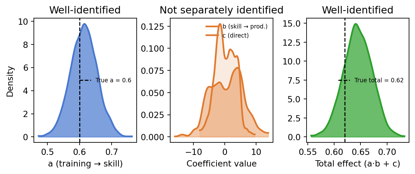

Figure 5: Left: the training → skill coefficient a is well-identified by sparse measurements (true value: dashed line). Centre: b and c are individually diffuse due to collinearity between the latent and its parent. Right: the total effect a·b + c is precisely estimated despite the individual non-identifiability.

Without measurements, the latent scale is unidentified

A deterministic latent M \equiv a \cdot X has an inherent scaling ambiguity: any rescaling M' = k \cdot M with a' = k \cdot a and b' = b/k leaves a \cdot b unchanged. Without at least one observation that pins down the scale of M, the sampler must explore a hyperbolic ridge in the (a, b) posterior — producing hundreds of divergences and poor mixing.

Even 5–10% coverage with moderate measurement noise can be enough to collapse the ridge. In this example, assessments for 30% of employees eliminate divergences entirely.

To separately identify b and c, the latent state needs independent variation beyond what X provides — either process noise (stochastic latent, families={"M": "latent_normal"}) or temporal dynamics (panel data with AR structure). The brand awareness example demonstrates fully identified models using stochastic latent states and survey-augmented measurement equations.

Total causal effect via do()

Despite the partial non-identifiability of individual paths, the do() operator correctly recovers the total causal effect:

ate3 = model3.ate("Y", "X")
print("True total effect: 0.620")
ate3

True total effect: 0.620

ATE of X on Y

Mean	0.64
94% HDI	[0.60, 0.70]
P(> 0)	1.00
Draws	4000

Methods: .hdi() .prob() .summary() .draws() .by_time() .dataset

Summary

Labeled coefficients and defined parameters (:=) let you name path coefficients and compute derived quantities like indirect effects, with full posterior uncertainty propagation.
effect("X -> M -> Y") computes path-specific effects by multiplying draws along a specified causal path.
Parallel mediators can be modelled by adding equations for each mediator and using ~~ to account for unmodeled common causes via an LKJ prior on residual correlations.
Latent mediators (latent=["M"]) encode causal mechanisms through unobserved variables. The model infers the latent state from upstream causes and downstream outcomes.
Sparse measurement equations (M_obs ~ 0 + 1*M) anchor the latent scale with even a small fraction of noisy observations, resolving a scaling ambiguity that otherwise causes sampling failures.
Total causal effects via do() remain well-identified even when individual path coefficients are not, because the total depends only on estimable combinations of parameters.
Sequential ignorability — no unmeasured common cause of mediator and outcome — is required for valid direct/indirect decomposition and is untestable from data alone.

Where might mediation analysis appear in your work?

Marketing: upper-funnel spend builds brand awareness (potentially latent), which drives conversions. Brand tracking surveys provide sparse measurements. Are the two channels’ awareness effects correlated through a shared audience trait?
Education: a curriculum redesign affects student engagement (mediator), which drives test scores. If engagement is only measured for a subset via classroom observations, a latent mediator model can recover the pathway.
Product: a UI change affects user comprehension (latent) and task completion (outcome). Sparse usability-test scores anchor the latent state.

In each case, ask: what is the mechanism through which the cause operates? Is that mechanism fully observed, partially observed, or shared across multiple pathways?