
Local Slopes on the Response Scale

Finite-difference slopes on the probability scale for a Bernoulli GLM with interaction, dydx vs eyex, and the adjustment-covariate warning.
Author

Benjamin Vincent

Goal: visualize how the local effect of ad spend on conversion changes with income on the response scale.

On a logistic model the coefficient on ad spend is a log-odds slope; slopes(wrt="ad_spend") returns \partial P(\text{converted}) / \partial \text{ad\_spend} via a finite difference under do(). With an ad_spend:income interaction, that derivative is a function of income, not a single number.

Prerequisites: Predictions, Comparisons, and Slopes; Treatment Effects with Non-Linear Models.

Setup

import numpy as np
import pandas as pd
import matplotlib.pyplot as plt
from scipy.special import expit
import pathmc

FIG_WIDTH = 7
FIG_HEIGHT = 4
COLOR_STRUCTURAL = "#2171b5"
COLOR_ADJUSTMENT = "#e6550d"
COLOR_TRUE = "#333333"
COLOR_WARNING = "#d62728"


def plot_hdi_line(x, samples, ax, color, hdi_prob=0.94, alpha=0.2, label=None):
    """Posterior mean with quantile band. samples shape (n_draws, n_points)."""
    lo_q = (1 - hdi_prob) / 2
    lower = np.quantile(samples, lo_q, axis=0)
    upper = np.quantile(samples, 1 - lo_q, axis=0)
    mean = samples.mean(axis=0)
    ax.fill_between(x, lower, upper, color=color, alpha=alpha, linewidth=0)
    ax.plot(x, mean, color=color, linewidth=2.5, label=label)
    return mean


TRUE_B0 = -0.3
TRUE_B_DOSE = 0.9
TRUE_B_INC = 0.5
TRUE_B_INT = 0.4
TRUE_B_SEG = 0.25

rng = np.random.default_rng(42)
n = 600

Shared dose-response scenario

income income ad_spend ad_spend income->ad_spend converted converted income->converted ad_spend->converted
Figure 1: Bernoulli dose-response with ad_spend:income interaction; local slope dP(converted)/d(ad_spend) varies with income.
income = rng.normal(0, 1, n)
ad_spend = 0.6 * income + rng.normal(0, 0.5, n)
segment = np.where(income < -0.5, 0.0, np.where(income < 0.5, 1.0, 2.0))


def true_dydx(ad_spend_val, income_val, segment_val=1.0):
    logit = (
        TRUE_B0
        + TRUE_B_DOSE * ad_spend_val
        + TRUE_B_INC * income_val
        + TRUE_B_INT * ad_spend_val * income_val
        + TRUE_B_SEG * segment_val
    )
    p = expit(logit)
    return p * (1 - p) * (TRUE_B_DOSE + TRUE_B_INT * income_val)


logit = (
    TRUE_B0
    + TRUE_B_DOSE * ad_spend
    + TRUE_B_INC * income
    + TRUE_B_INT * ad_spend * income
    + TRUE_B_SEG * segment
)
converted = rng.binomial(1, expit(logit)).astype(float)
df = pd.DataFrame({
    "income": income,
    "ad_spend": ad_spend,
    "segment": segment,
    "converted": converted,
})

spec = """
ad_spend ~ income
converted ~ ad_spend + income + ad_spend:income + segment
"""
scm = pathmc.model(spec, data=df, families={"converted": "bernoulli"})
scm.fit(random_seed=42)
adj = scm.adjustment_model("ad_spend -> converted")
adj.fit(random_seed=42)
Initializing NUTS using jitter+adapt_diag...
Multiprocess sampling (4 chains in 4 jobs)
NUTS: [beta_converted, sigma_ad_spend, beta_ad_spend]

Sampling 4 chains for 1_000 tune and 1_000 draw iterations (4_000 + 4_000 draws total) took 4 seconds.
Initializing NUTS using jitter+adapt_diag...
Multiprocess sampling (4 chains in 4 jobs)
NUTS: [beta_converted]

Sampling 4 chains for 1_000 tune and 1_000 draw iterations (4_000 + 4_000 draws total) took 3 seconds.
<xarray.DataTree>
Group: /
├── Group: /posterior
│       Dimensions:               (chain: 4, draw: 1000, converted_predictors: 3,
│                                  mu_converted_dim_0: 600)
│       Coordinates:
│         * chain                 (chain) int64 32B 0 1 2 3
│         * draw                  (draw) int64 8kB 0 1 2 3 4 5 ... 995 996 997 998 999
│         * converted_predictors  (converted_predictors) <U9 108B 'Intercept' ... 'in...
│         * mu_converted_dim_0    (mu_converted_dim_0) int64 5kB 0 1 2 3 ... 597 598 599
│       Data variables:
│           beta_converted        (chain, draw, converted_predictors) float64 96kB -0...
│           mu_converted          (chain, draw, mu_converted_dim_0) float64 19MB 0.33...
│       Attributes:
│           created_at:                 2026-09-30T20:17:47.452345+00:00
│           creation_library:           ArviZ
│           creation_library_version:   1.2.0
│           creation_library_language:  Python
│           inference_library:          pymc
│           inference_library_version:  6.2.0
│           sample_dims:                ['chain', 'draw']
│           sampling_time:              2.7571818828582764
│           tuning_steps:               1000
├── Group: /sample_stats
│       Dimensions:                (chain: 4, draw: 1000)
│       Coordinates:
│         * chain                  (chain) int64 32B 0 1 2 3
│         * draw                   (draw) int64 8kB 0 1 2 3 4 5 ... 995 996 997 998 999
│       Data variables: (12/18)
│           process_time_diff      (chain, draw) float64 32kB 0.000371 ... 0.00028
│           max_energy_error       (chain, draw) float64 32kB 0.7974 -0.9956 ... 0.2492
│           perf_counter_start     (chain, draw) float64 32kB 1.084e+06 ... 1.084e+06
│           tree_depth             (chain, draw) int64 32kB 3 2 2 2 3 2 ... 1 2 2 3 2 2
│           diverging              (chain, draw) bool 4kB False False ... False False
│           divergences            (chain, draw) int64 32kB 0 0 0 0 0 0 ... 0 0 0 0 0 0
│           ...                     ...
│           step_size_bar          (chain, draw) float64 32kB 0.8628 0.8628 ... 0.818
│           perf_counter_diff      (chain, draw) float64 32kB 0.0003788 ... 0.0002841
│           index_in_trajectory    (chain, draw) int64 32kB 6 -2 -1 -2 -5 ... 1 2 -2 -3
│           reached_max_treedepth  (chain, draw) bool 4kB False False ... False False
│           largest_eigval         (chain, draw) float64 32kB nan nan nan ... nan nan
│           energy_error           (chain, draw) float64 32kB 0.3502 0.1365 ... 0.2492
│       Attributes:
│           created_at:                 2026-09-30T20:17:47.459317+00:00
│           creation_library:           ArviZ
│           creation_library_version:   1.2.0
│           creation_library_language:  Python
│           inference_library:          pymc
│           inference_library_version:  6.2.0
│           sample_dims:                ['chain', 'draw']
│           sampling_time:              2.7571818828582764
│           tuning_steps:               1000
├── Group: /observed_data
│       Dimensions:          (converted_dim_0: 600)
│       Coordinates:
│         * converted_dim_0  (converted_dim_0) int64 5kB 0 1 2 3 4 ... 596 597 598 599
│       Data variables:
│           converted        (converted_dim_0) int64 5kB 1 0 1 1 1 0 1 ... 0 0 0 0 1 1 0
│       Attributes:
│           created_at:                 2026-09-30T20:17:47.461410+00:00
│           creation_library:           ArviZ
│           creation_library_version:   1.2.0
│           creation_library_language:  Python
│           inference_library:          pymc
│           inference_library_version:  6.2.0
│           sample_dims:                []
├── Group: /constant_data
│       Dimensions:         (income_dim_0: 600, ad_spend_dim_0: 600)
│       Coordinates:
│         * income_dim_0    (income_dim_0) int64 5kB 0 1 2 3 4 5 ... 595 596 597 598 599
│         * ad_spend_dim_0  (ad_spend_dim_0) int64 5kB 0 1 2 3 4 ... 595 596 597 598 599
│       Data variables:
│           income          (income_dim_0) float64 5kB 0.3047 -1.04 ... 0.2417 -1.775
│           ad_spend        (ad_spend_dim_0) float64 5kB 0.4405 -0.9128 ... -1.594
│       Attributes:
│           created_at:                 2026-09-30T20:17:47.462291+00:00
│           creation_library:           ArviZ
│           creation_library_version:   1.2.0
│           creation_library_language:  Python
│           inference_library:          pymc
│           inference_library_version:  6.2.0
│           sample_dims:                []
└── Group: /log_likelihood
        Dimensions:          (chain: 4, draw: 1000, converted_dim_0: 600)
        Coordinates:
          * chain            (chain) int64 32B 0 1 2 3
          * draw             (draw) int64 8kB 0 1 2 3 4 5 6 ... 994 995 996 997 998 999
          * converted_dim_0  (converted_dim_0) int64 5kB 0 1 2 3 4 ... 596 597 598 599
        Data variables:
            converted        (chain, draw, converted_dim_0) float64 19MB -0.5382 ... ...
        Attributes:
            created_at:                 2026-09-30T20:17:47.593880+00:00
            creation_library:           ArviZ
            creation_library_version:   1.2.0
            creation_library_language:  Python
            inference_library:          pymc
            inference_library_version:  6.2.0
            sample_dims:                ['chain', 'draw']

Treatment slope vs income

We evaluate slopes on a grid by finite-differencing interventional predictions (same logic as slopes()).

income_grid = np.linspace(-2.0, 2.0, 25)
dose_ref = 0.0
eps = 1e-4
grid = pathmc.datagrid(df, ad_spend=[dose_ref], income=income_grid, segment=[1.0])
grid_hi = grid.assign(ad_spend=dose_ref + eps)

lo = scm.predictions(
    "converted", set={"ad_spend": grid["ad_spend"].values}, newdata=grid
)
hi = scm.predictions(
    "converted", set={"ad_spend": grid_hi["ad_spend"].values}, newdata=grid_hi
)
slope_da = (hi.dataset["converted"] - lo.dataset["converted"]) / eps
Code
fig, ax = plt.subplots(figsize=(FIG_WIDTH, FIG_HEIGHT))
x = grid["income"].values
samples = slope_da.stack(sample=("chain", "draw")).values.T
plot_hdi_line(x, samples, ax, color=COLOR_STRUCTURAL, alpha=0.2, label="posterior mean")
ax.plot(
    x,
    true_dydx(dose_ref, x),
    color=COLOR_TRUE,
    linestyle="--",
    linewidth=1.5,
    label="true",
)
ax.set_xlabel("income")
ax.set_ylabel("dP(converted)/d(ad_spend)")
ax.legend(frameon=False)
plt.tight_layout()
plt.show()
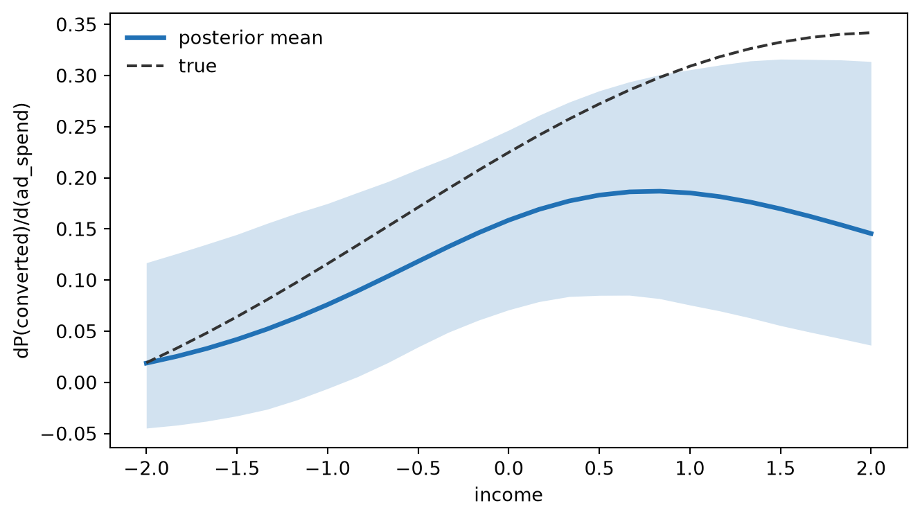
Figure 2: Local slope dP(converted)/d(ad_spend) at ad_spend=0 vs income (segment=1), structural model, 94% HDI; true derivative black dashed.

If this curve were flat, the interaction would be doing no work on the response scale; the bend is the point of the notebook.

Slopes table

slope_table = []
for inc in [-1.0, 0.0, 1.0]:
    result = scm.slopes(
        "converted",
        "ad_spend",
        slope="dydx",
        conditional={"income": inc, "segment": 1.0},
        average_by="all",
    )
    lo, hi = result.hdi(prob=0.94)
    slope_table.append({
        "wrt": "ad_spend",
        "income": inc,
        "segment": 1,
        "mean": result.mean(),
        "hdi_low": lo,
        "hdi_high": hi,
        "causal": result.causal,
    })

pd.DataFrame(slope_table)
wrt income segment mean hdi_low hdi_high causal
0 ad_spend -1.0 1 0.074127 -0.013427 0.156994 True
1 ad_spend 0.0 1 0.149200 0.072782 0.221372 True
2 ad_spend 1.0 1 0.173612 0.079192 0.265460 True

dydx vs eyex

dydx = scm.slopes("converted", "ad_spend", slope="dydx", average_by="all")
eyex = scm.slopes("converted", "ad_spend", slope="eyex", average_by="all")
pd.DataFrame([
    {
        "slope": "dydx",
        "mean": dydx.mean(),
        "hdi_low": dydx.hdi()[0],
        "hdi_high": dydx.hdi()[1],
    },
    {
        "slope": "eyex",
        "mean": eyex.mean(),
        "hdi_low": eyex.hdi()[0],
        "hdi_high": eyex.hdi()[1],
    },
])
slope mean hdi_low hdi_high
0 dydx 0.120386 0.055158 0.186081
1 eyex -0.036499 -0.121422 0.049315
WarningLocal positivity and eps

slopes() uses a symmetric finite difference at wrt and wrt + eps. If wrt + eps leaves the support of the data or drives predicted probabilities to 0 or 1, the derivative can be unstable. Inspect slopes on a datagrid() when reporting derivatives far from the bulk of the data.

Adjustment covariate slope is not a treatment effect

On AdjustmentModel, slopes(wrt="income") is interventional on the reduced equation but causal=False because income is an adjustment variable, not the designated treatment.

Code
slope_treat = adj.slopes(slope="dydx", average_by="all")
slope_conf = adj.slopes(wrt="income", slope="dydx", average_by="all")

fig, ax = plt.subplots(figsize=(FIG_WIDTH, FIG_HEIGHT * 0.85))
bars = [
    ("ad_spend (treatment)", slope_treat.mean(), slope_treat.causal, COLOR_STRUCTURAL),
    ("income (adjustment)", slope_conf.mean(), slope_conf.causal, COLOR_WARNING),
]
for i, (label, mean, causal, color) in enumerate(bars):
    ax.bar(i, mean, color=color, alpha=0.85)
    ax.text(i, mean + 0.005, f"causal={causal}", ha="center", fontsize=9)

ax.set_xticks(range(len(bars)))
ax.set_xticklabels([b[0] for b in bars])
ax.set_ylabel("dP(converted)/d(wrt)")
plt.tight_layout()
plt.show()
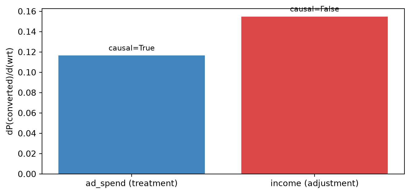
Figure 3: AdjustmentModel slope wrt income (red): interventional fit on the outcome surface but causal=False; treatment slope wrt ad_spend (blue): causal=True.

Do not report the red bar as the causal effect of income on conversion.

Structural vs adjustment treatment slopes

Code
fig, ax = plt.subplots(figsize=(FIG_WIDTH, FIG_HEIGHT * 0.85))
for model, color, label in [
    (scm, COLOR_STRUCTURAL, "structural"),
    (adj, COLOR_ADJUSTMENT, "adjustment"),
]:
    if label == "structural":
        result = model.slopes("converted", "ad_spend", slope="dydx", average_by="all")
    else:
        result = model.slopes(slope="dydx", average_by="all")
    lo, hi = result.hdi(prob=0.94)
    ax.errorbar(
        label,
        result.mean(),
        yerr=[[result.mean() - lo], [hi - result.mean()]],
        fmt="o",
        color=color,
        markersize=10,
        capsize=5,
        linewidth=2,
    )

ax.set_ylabel("dP(converted)/d(ad_spend)")
plt.tight_layout()
plt.show()
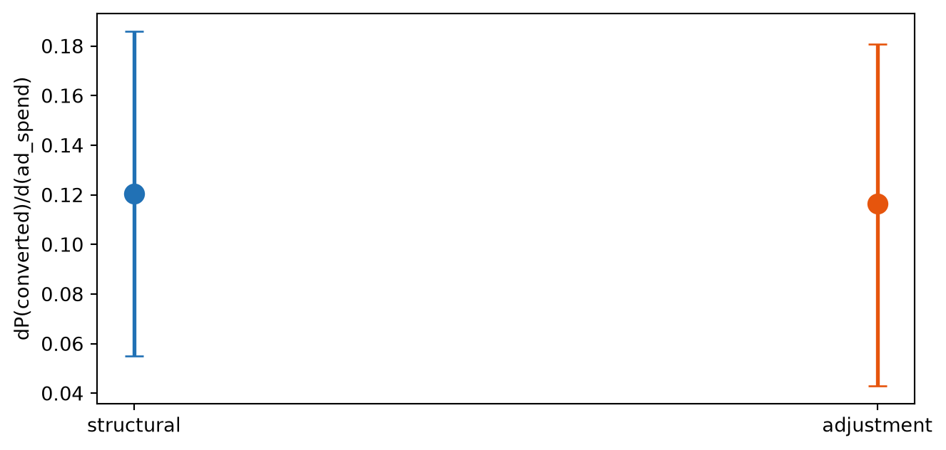
Figure 4: Population-average treatment slope dP(converted)/d(ad_spend): structural (blue) vs adjustment (orange) posterior means with 94% HDI error bars.

Unit-level slopes, then average

unit_slopes = scm.slopes("converted", "ad_spend", slope="dydx", average_by=None)
pop_slope = scm.slopes("converted", "ad_spend", slope="dydx", average_by="all")
print(
    f"mean of unit slopes: {unit_slopes.dataset['converted'].mean(dim=('chain', 'draw', 'unit')):.4f}"
)
print(f"average_by=all:      {pop_slope.mean():.4f}")
mean of unit slopes: 0.1204
average_by=all:      0.1204

Summary

  • On a GLM, slopes() answers on the response scale; the coefficient is not interchangeable.
  • Interactions make the slope a function of conditioning covariates.
  • Check causal on AdjustmentModel slopes before narrating adjustment variables as treatments.
  • dydx and eyex summarize different economic questions; pick deliberately.

Next steps: Conditional Predictions; Interventional Contrasts; Predictions, Comparisons, and Slopes; SCM vs Regression Adjustment.

NoteReflection

For a continuous price or dose lever in your work, is the local slope near typical values more actionable than a two-point ATE? Which covariates in your adjustment set would be dangerous to report as if they were treatments?