Custom Transforms

Define domain-specific nonlinearities with estimable parameters and use them in the pathmc DSL.

Author

Benjamin Vincent

pathmc ships with adstock and logistic_saturation for marketing mix models, but many domains need different functional forms. A pharmacologist modeling dose-response needs a Hill function; an ecologist modeling growth needs a Monod curve; a psychophysicist modeling perception needs a Weibull function. The transform registry lets you define exactly the nonlinearity your domain requires, with parameters estimated jointly alongside the structural coefficients.

This tutorial walks through the full lifecycle: define a custom transform, register it, use it in the DSL, fit, and verify that do() recomputes the transform correctly under interventions.

The scenario: dose-response with a Hill function

A researcher runs a dose-response experiment: subjects receive different doses of a compound and their response is measured. The relationship is nonlinear — response saturates at high doses — and the specific shape follows the Hill equation:

f(x; n, K) = \frac{x^n}{K^n + x^n}

where K is the dose at which response reaches half its maximum (the EC50), and n controls the steepness of the curve (the Hill coefficient). Neither of pathmc’s built-in transforms captures this shape, so we need a custom one.

Figure 1: Causal structure: dose determines response via a Hill-shaped nonlinearity. The transform parameters n and K are estimated from data.

Step 1: Define the transform

A custom transform subclasses Transform and provides three things:

name — the identifier used in the DSL
param_specs — a dict mapping parameter names to ParamSpec objects that declare constraints and default priors
apply_pymc() — the forward computation using PyTensor-compatible operations

from pathmc.transforms import Transform, ParamSpec, register_transform


class Hill(Transform):
    """Hill saturation: f(x; n, K) = x^n / (K^n + x^n)."""

    name = "hill"
    param_specs = {
        "n": ParamSpec(constraint="positive", default_prior="HalfNormal(1)"),
        "K": ParamSpec(constraint="positive", default_prior="HalfNormal(1)"),
    }

    def apply_pymc(self, x, params, *, panel_info=None, data=None):
        n = params["n"]
        K = params["K"]
        return x**n / (K**n + x**n)

How constraints map to default priors

The constraint field in ParamSpec determines the automatic prior:

Constraint	Default prior	Support
`"positive"`	`HalfNormal(sigma=1)`	(0, \infty)
`"unit_interval"`	`Beta(alpha=2, beta=2)`	(0, 1)
anything else	`Normal(mu=0, sigma=10)`	(-\infty, \infty)

These defaults are reasonable starting points. For domain-specific knowledge, override them via priors={} at fit time — just like any other model parameter (see Custom Priors).

The Hill transform is pointwise — each observation is transformed independently, with no dependence on previous time steps. That means we can use the default has_state = False and step() implementations inherited from Transform. Transforms that carry state across time (like adstock) would override these; see the built-in Adstock implementation for an example.

Step 2: Register and use in the DSL

Registration makes the transform available by name in the model specification string.

register_transform(Hill())

Once registered, the transform works like any built-in — same DSL syntax, same prior introspection, same do() support.

Simulate data with known parameters

To verify the transform works correctly, we generate data from a known Hill curve and check that pathmc recovers the true parameters.

import numpy as np
import pandas as pd

rng = np.random.default_rng(42)
n_obs = 200

TRUE_N = 2.0
TRUE_K = 5.0
TRUE_B = 100.0
TRUE_SIGMA = 3.0

dose = rng.uniform(0.5, 20, size=n_obs)
hill_value = dose**TRUE_N / (TRUE_K**TRUE_N + dose**TRUE_N)
response = TRUE_B * hill_value + rng.normal(0, TRUE_SIGMA, size=n_obs)

df = pd.DataFrame({"dose": dose, "response": response})

True values: n = 2, K = 5, b = 100, \sigma = 3.

Code

import matplotlib.pyplot as plt

FIG_WIDTH = 7
FIG_HEIGHT = 3.5

COLOR_DATA = "#bdbdbd"
COLOR_TRUE = "black"
COLOR_POSTERIOR = "#d95f02"

Code

dose_grid = np.linspace(0.5, 20, 200)
true_curve = TRUE_B * dose_grid**TRUE_N / (TRUE_K**TRUE_N + dose_grid**TRUE_N)

fig, ax = plt.subplots(figsize=(FIG_WIDTH, FIG_HEIGHT))
ax.scatter(
    df["dose"],
    df["response"],
    color=COLOR_DATA,
    s=15,
    alpha=0.6,
    label="Observed data",
    zorder=2,
)
ax.plot(
    dose_grid,
    true_curve,
    color=COLOR_TRUE,
    linestyle="--",
    linewidth=2,
    label="True Hill curve",
    zorder=3,
)
ax.set_xlabel("Dose")
ax.set_ylabel("Response")
ax.legend()
plt.tight_layout()
plt.show()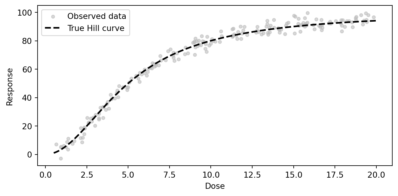

Figure 2: Simulated dose-response data (grey) with the true Hill curve (black dashed). The curve saturates near the maximum response of 100 as dose increases.

Fit the model

The DSL syntax for transforms follows the pattern transform_name(variable, param1=name1, param2=name2). The parameter names on the right-hand side of = become the names of the estimated quantities in the posterior.

import pathmc
from pathmc import Prior

spec = "response ~ b * hill(dose, n=n, K=K)"

model = pathmc.model(
    spec,
    data=df,
    priors={
        "n": Prior("HalfNormal", sigma=3),
        "K": Prior("HalfNormal", sigma=10),
    },
)

Why override the default priors?

The default HalfNormal(sigma=1) for both n and K would concentrate mass near zero — fine as a generic starting point, but we know that K is measured in dose units (plausibly 1–20) and n is typically 1–4 in pharmacology. Wider priors let the data speak without forcing unrealistically small values.

model.equations()

\begin{aligned} \beta_{response} &\sim \text{Normal}(mu=0,\, sigma=10) \\ \sigma_{response} &\sim \text{HalfNormal}(sigma=1) \\ n &\sim \text{HalfNormal}(sigma=3) \\ K &\sim \text{HalfNormal}(sigma=10) \\[6pt] \mu_{response} &= \beta_{0,\,response} + b \cdot \operatorname{hill}(\mathrm{dose},\, n,\, K) \\ \mathrm{response} &\sim \text{Normal}(\mu_{response},\, \sigma_{response}) \end{aligned}

The equations and priors show both the structural parameters (b, sigma_response) and the transform parameters (n, K). Transform parameters are first-class model parameters — they appear in the posterior, respond to set_priors(), and propagate uncertainty through do().

idata = model.fit(draws=500, tune=500, chains=4, random_seed=42)

NUTS[nutpie]: [n, K, beta_response, sigma_response]

Parameter recovery

model.effects_summary()

	mean	sd	hdi_3%	hdi_97%
name
b	96.170806	1.782753	92.754813	99.552759

Code

import arviz as az

az.plot_dist(
    idata,
    var_names=["n", "K"],
    ci_kind="hdi",
    ci_prob=0.94,
    visuals={"title": False, "point_estimate_text": False},
    figure_kwargs={"figsize": (FIG_WIDTH, FIG_HEIGHT)},
)
for ax, true_val, label in zip(
    plt.gcf().axes,
    [TRUE_N, TRUE_K],
    ["n (Hill coefficient)", "K (EC50)"],
):
    ax.axvline(true_val, color="k", ls="--", lw=1.5)
    ax.set_xlabel(label)
plt.tight_layout()
plt.show()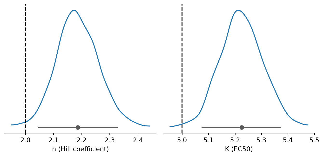

Figure 3: Posterior distributions for the Hill parameters n and K, with true values (black dashed). Both parameters are well-recovered.

Interventional predictions with do()

The real payoff of a custom transform is that do() recomputes it automatically. When we intervene on dose, the Hill function is re-evaluated at the new dose using posterior draws of n and K, propagating parameter uncertainty through the nonlinearity.

dose_grid_do = np.linspace(0.5, 20, 30)

response_draws_list = []
for d in dose_grid_do:
    result = model.do(set={"dose": d})
    response_draws_list.append(result.draws("response"))

response_draws_2d = np.column_stack(response_draws_list)
means = response_draws_2d.mean(axis=0)

/var/folders/pd/p2qnky2x3xl4w3mgc4lct2200000gn/T/ipykernel_85523/2654734205.py:5: UserWarning: Intervention value 0.50 for 'dose' is outside the observed data range [0.64, 19.85]. Results are extrapolations and should be interpreted with caution.
  result = model.do(set={"dose": d})
/var/folders/pd/p2qnky2x3xl4w3mgc4lct2200000gn/T/ipykernel_85523/2654734205.py:5: UserWarning: Intervention value 20.00 for 'dose' is outside the observed data range [0.64, 19.85]. Results are extrapolations and should be interpreted with caution.
  result = model.do(set={"dose": d})

Code

fig, ax = plt.subplots(figsize=(FIG_WIDTH, FIG_HEIGHT))

hdi_1 = az.hdi(response_draws_2d, prob=0.94, axis=0)
ax.fill_between(
    dose_grid_do,
    hdi_1[:, 0],
    hdi_1[:, 1],
    alpha=0.3,
    color=COLOR_POSTERIOR,
    label="94% HDI",
)
ax.plot(
    dose_grid_do,
    means,
    color=COLOR_POSTERIOR,
    linewidth=2,
    label="Posterior mean",
    zorder=3,
)
ax.plot(
    dose_grid,
    true_curve,
    color=COLOR_TRUE,
    linestyle="--",
    linewidth=1.5,
    label="True curve",
    zorder=4,
)
ax.scatter(df["dose"], df["response"], color=COLOR_DATA, s=10, alpha=0.4, zorder=1)
ax.set_xlabel("Dose")
ax.set_ylabel("Response")
ax.legend()
plt.tight_layout()
plt.show()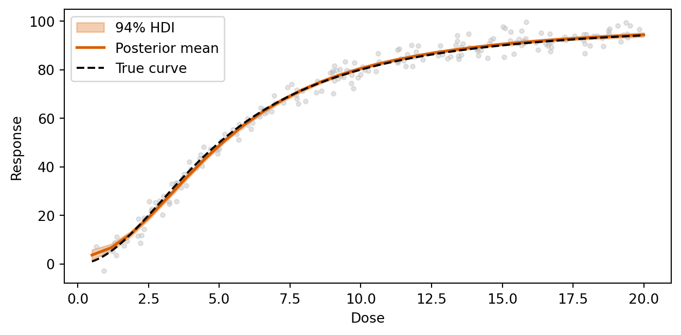

Figure 4: Posterior predictive response curve under do(dose = d) for a range of doses. The orange band shows the 94% HDI; the true curve is recovered with appropriate uncertainty.

The do() curve closely tracks the true Hill function, with the HDI band widening where data is sparse. This is the standard Bayesian behavior: uncertainty grows where the model has less information.

Answering causal questions

With the fitted model, we can answer dose-comparison questions directly. For example: what is the expected gain in response from increasing dose from 2 to 10?

baseline = model.do(set={"dose": 2})
increased = model.do(set={"dose": 10})
contrast = increased - baseline

print(
    f"Expected response at dose=2:  {baseline.mean('response'):.1f}  "
    f"{baseline.hdi('response')}"
)
print(
    f"Expected response at dose=10: {increased.mean('response'):.1f}  "
    f"{increased.hdi('response')}"
)
print(
    f"Causal effect of dose 2→10:   {contrast.mean('response'):.1f}  "
    f"{contrast.hdi('response')}"
)

Expected response at dose=2:  13.6  [12.50253141 14.61596433]
Expected response at dose=10: 80.5  [79.88910174 81.09798829]
Causal effect of dose 2→10:   66.9  [65.5186103  68.14100273]

The contrast gives the full posterior distribution of the causal effect, including uncertainty from all model parameters — the coefficient b, the Hill parameters n and K, and the residual noise.

Summary

Subclass Transform with a name, param_specs dict, and apply_pymc() method. The method receives PyTensor tensors and must return a tensor.
ParamSpec declares the constraint ("positive", "unit_interval") and a human-readable default prior string. The constraint determines the automatic prior distribution.
register_transform() makes the transform available in the DSL. Call it before pathmc.model().
DSL syntax is transform_name(variable, param=name). Parameter names become posterior quantities with full uncertainty.
Priors for transform parameters can be overridden via priors={} at fit time, just like structural coefficients.
do() recomputes the transform under interventions automatically — no extra code needed. Parameter uncertainty propagates through the nonlinearity.
Pointwise transforms (no temporal dependence) only need apply_pymc(). For stateful transforms (carry-over effects), override has_state and step().

Bring your own nonlinearity

What functional forms matter in your domain? A few candidates:

Pharmacology: Michaelis-Menten kinetics (v = V_{\max} \cdot [S] / (K_m + [S])) — structurally identical to Hill with n = 1.
Ecology: Monod growth (\mu = \mu_{\max} \cdot S / (K_s + S)) for nutrient-limited growth curves.
Psychophysics: power-law transforms (y = x^\alpha) for Stevens’ law, where a single estimable exponent captures the perceptual nonlinearity.
Economics: CES production functions with estimable elasticity of substitution.

Each of these is a few lines of apply_pymc() away from a working pathmc transform.