Placebo Refutation

Swap the treatment for a permuted copy and re-fit: a sound pipeline must report no effect. When it reports one anyway, the estimate was never yours to keep.

Author

Carlos Trujillo

Your model fits, the ATE is comfortably away from zero, and the DAG survived falsification. One question remains: does the pipeline itself — spec, priors, likelihood, sampler, and estimand all together — manufacture effects out of nothing?

The placebo test answers it by breaking the thing you claim to measure. Permute the treatment column and the treatment can no longer cause the outcome: whatever structural link existed is severed by the shuffle. Re-fit on that sabotaged data and a sound pipeline must come back empty-handed. If it still reports an effect, the number it gave you on the real data was partly an artifact of the machinery, not evidence from the world.

This page assumes you have read Treatment Effects with Non-Linear Models, which covers ate() and g-computation, and ideally Causal Identification for the backdoor/confounding setup used below. You need to be comfortable with what an ATE is before it makes sense to ask whether yours is real.

This is the Bayesian upgrade of DoWhy’s placebo_treatment_refuter (Sharma and Kiciman 2020). Because every re-fit yields a full posterior rather than a point estimate, pathmc pools the per-permutation summaries through a hierarchical normal-normal model — think of it as meta-analysing the placebo re-fits, treating each shuffle as one study. That pooling separates two things a point estimate confounds: the systematic placebo bias \mu_\text{null} (should straddle zero) and the structural volatility \tau_\text{het} (how much the estimate wobbles between shuffles). The real effect is then calibrated against the resulting null. The calibration model follows Bugaev and Trujillo (n.d.).

Setup

import numpy as np
import pandas as pd
import matplotlib.pyplot as plt
import pathmc
from pathmc import Prior

FIG_WIDTH = 8
FIG_HEIGHT = 4

# Each permutation is a full MCMC re-fit, so keep the per-fit cost modest.
FIT = {"draws": 500, "tune": 500, "chains": 2}
REFIT = {"draws": 500, "tune": 500, "chains": 2}

An estimate worth stress-testing

A treatment X, an outcome Y, and an observed confounder Z that drives both. The true causal effect of X on Y is 0.5, and adjusting for Z identifies it.

Figure 1: Z confounds the X–Y relationship. Adjusting for Z identifies the causal effect of X on Y.

def make_data(true_effect, n, noise, seed):
    """Confounded X -> Y data with an observed confounder Z."""
    rng = np.random.default_rng(seed)
    Z = rng.normal(size=n)
    X = 0.6 * Z + rng.normal(scale=0.5, size=n)
    Y = true_effect * X + 0.8 * Z + rng.normal(scale=noise, size=n)
    return pd.DataFrame({"X": X, "Y": Y, "Z": Z})


true_effect = 0.5
df = make_data(true_effect, n=500, noise=0.5, seed=42)

spec = """
X ~ a*Z
Y ~ b*X + c*Z
"""

model = pathmc.model(spec, data=df)
model.fit(random_seed=42, **FIT)

NUTS[nutpie]: [beta_Y, sigma_X, beta_X, sigma_Y]

<xarray.DataTree>
Group: /
├── Group: /posterior
│       Dimensions:       (chain: 2, draw: 500, Y_predictors: 3, X_predictors: 2,
│                          mu_Y_dim_0: 500, mu_X_dim_0: 500)
│       Coordinates:
│         * chain         (chain) int64 16B 0 1
│         * draw          (draw) int64 4kB 0 1 2 3 4 5 6 ... 493 494 495 496 497 498 499
│         * Y_predictors  (Y_predictors) object 24B 'Intercept' 'X' 'Z'
│         * X_predictors  (X_predictors) object 16B 'Intercept' 'Z'
│         * mu_Y_dim_0    (mu_Y_dim_0) int64 4kB 0 1 2 3 4 5 ... 494 495 496 497 498 499
│         * mu_X_dim_0    (mu_X_dim_0) int64 4kB 0 1 2 3 4 5 ... 494 495 496 497 498 499
│       Data variables:
│           beta_Y        (chain, draw, Y_predictors) float64 24kB -0.02869 ... 0.8714
│           beta_X        (chain, draw, X_predictors) float64 16kB 0.02253 ... 0.6064
│           sigma_X       (chain, draw) float64 8kB 0.5186 0.5098 ... 0.4911 0.5048
│           sigma_Y       (chain, draw) float64 8kB 0.5024 0.5165 ... 0.5182 0.4988
│           mu_Y          (chain, draw, mu_Y_dim_0) float64 4MB 0.6409 ... -1.529
│           mu_X          (chain, draw, mu_X_dim_0) float64 4MB 0.2048 ... -0.942
│       Attributes:
│           created_at:                 2026-08-06T11:58:49.355719+00:00
│           creation_library:           ArviZ
│           creation_library_version:   1.1.0
│           creation_library_language:  Python
│           sample_dims:                ['chain', 'draw']
│           inference_library:          nutpie
│           inference_library_version:  0.16.10
│           sampling_time:              0.10490179061889648
│           tuning_steps:               500
├── Group: /sample_stats
│       Dimensions:                   (chain: 2, draw: 500)
│       Coordinates:
│         * chain                     (chain) int64 16B 0 1
│         * draw                      (draw) int64 4kB 0 1 2 3 4 ... 495 496 497 498 499
│       Data variables: (12/20)
│           depth                     (chain, draw) uint64 8kB 3 3 3 2 2 3 ... 2 3 2 3 3
│           maxdepth_reached          (chain, draw) bool 1kB False False ... False False
│           step_size                 (chain, draw) float64 8kB 0.7354 0.7572 ... 0.8202
│           transformation_update_id  (chain, draw) int64 8kB 0 0 0 0 0 0 ... 0 0 0 0 0
│           step_size_bar             (chain, draw) float64 8kB 0.7676 0.7676 ... 0.7658
│           mean_tree_accept          (chain, draw) float64 8kB 0.4049 0.8758 ... 0.9494
│           ...                        ...
│           fisher_distance           (chain, draw) float64 8kB 0.2736 0.4647 ... 0.9199
│           transformation_index      (chain, draw) int64 8kB 422 422 422 ... 423 423
│           diverging                 (chain, draw) bool 1kB False False ... False False
│           divergence_draw           (chain, draw) uint64 8kB 0 0 0 0 0 0 ... 0 0 0 0 0
│           divergence_message        (chain, draw) object 8kB None None ... None None
│           divergence_energy_error   (chain, draw) float64 8kB nan nan nan ... nan nan
│       Attributes:
│           created_at:                  2026-08-06T11:58:49.349045+00:00
│           creation_library:            ArviZ
│           creation_library_version:    1.1.0
│           creation_library_language:   Python
│           sample_dims:                 ['chain', 'draw']
│           inference_library:           nutpie
│           inference_library_version:   0.16.10
│           inference_library_settings:  {"sampler": "nuts", "adaptation": "diag", "s...
├── Group: /constant_data
│       Dimensions:  (Z_dim_0: 500)
│       Coordinates:
│         * Z_dim_0  (Z_dim_0) int64 4kB 0 1 2 3 4 5 6 7 ... 493 494 495 496 497 498 499
│       Data variables:
│           Z        (Z_dim_0) float64 4kB 0.3047 -1.04 0.7505 ... -0.3356 -1.991 -1.495
│       Attributes:
│           created_at:                 2026-08-06T11:58:49.352932+00:00
│           creation_library:           ArviZ
│           creation_library_version:   1.1.0
│           creation_library_language:  Python
│           inference_library:          pymc
│           inference_library_version:  6.0.1
│           sample_dims:                []
├── Group: /observed_data
│       Dimensions:  (X_dim_0: 500, Y_dim_0: 500)
│       Coordinates:
│         * X_dim_0  (X_dim_0) int64 4kB 0 1 2 3 4 5 6 7 ... 493 494 495 496 497 498 499
│         * Y_dim_0  (Y_dim_0) int64 4kB 0 1 2 3 4 5 6 7 ... 493 494 495 496 497 498 499
│       Data variables:
│           X        (X_dim_0) float64 4kB 0.8648 -0.1764 0.09053 ... -1.129 -0.4852
│           Y        (Y_dim_0) float64 4kB 0.6465 -1.285 0.4384 ... -1.801 -2.029
│       Attributes:
│           created_at:                 2026-08-06T11:58:49.354726+00:00
│           creation_library:           ArviZ
│           creation_library_version:   1.1.0
│           creation_library_language:  Python
│           inference_library:          pymc
│           inference_library_version:  6.0.1
│           sample_dims:                []
└── Group: /log_likelihood
        Dimensions:  (chain: 2, draw: 500, X_dim_0: 500, Y_dim_0: 500)
        Coordinates:
          * chain    (chain) int64 16B 0 1
          * draw     (draw) int64 4kB 0 1 2 3 4 5 6 7 ... 493 494 495 496 497 498 499
          * X_dim_0  (X_dim_0) int64 4kB 0 1 2 3 4 5 6 7 ... 493 494 495 496 497 498 499
          * Y_dim_0  (Y_dim_0) int64 4kB 0 1 2 3 4 5 6 7 ... 493 494 495 496 497 498 499
        Data variables:
            X        (chain, draw, X_dim_0) float64 4MB -1.072 -0.5955 ... -0.6448
            Y        (chain, draw, Y_dim_0) float64 4MB -0.2307 -0.4036 ... -0.7267
        Attributes:
            created_at:                 2026-08-06T11:58:49.466955+00:00
            creation_library:           ArviZ
            creation_library_version:   1.1.0
            creation_library_language:  Python
            inference_library:          pymc
            inference_library_version:  6.0.1
            sample_dims:                ['chain', 'draw']

ate = model.ate("Y", "X")
print(f"True effect: {true_effect}")
ate

True effect: 0.5

ATE of X on Y

Mean	0.46
94% HDI	[0.38, 0.55]
P(> 0)	1.00
Draws	1000

Methods: .hdi() .prob() .summary() .draws() .by_time() .dataset

That is a reality check worth pausing on: we simulated the data, so we know the answer is 0.5, and the model came back with 0.464 and a credible interval excluding zero. The workflow recovers what it should on data we control, which is the precondition for trusting it anywhere else. Now let’s find out whether that number is there because of the data or because of the pipeline.

Running the placebo test

refute_placebo() needs the outcome and the treatment to permute. Every permutation triggers a full re-fit, so sample_kwargs is forwarded to each one, and random_seed makes the whole thing reproducible.

refutation = model.refute_placebo(
    "Y",
    "X",
    n_permutations=4,
    sample_kwargs=REFIT,
    random_seed=101,
)
refutation

NUTS[nutpie]: [beta_Y, sigma_X, beta_X, sigma_Y]
NUTS[nutpie]: [beta_Y, sigma_X, beta_X, sigma_Y]
NUTS[nutpie]: [beta_Y, sigma_X, beta_X, sigma_Y]
NUTS[nutpie]: [beta_Y, sigma_X, beta_X, sigma_Y]
NUTS[nutpie]: [mu_null, tau_het, z]
Sampling: [theta_new]

Placebo Refutation: X → Y (α = 0.05)

Placebo test	✓ Pass — the placebo null straddles zero.
Real effect	✓ Survives — the observed effect is too extreme for placebo noise.
Placebo bias μ_null	0.0098 [-0.0434, 0.0587]
Structural volatility τ_het	0.0352
Observed ATE	0.4640 [0.3826, 0.5512]
Calibration	z = 6.180, p_tail = 0.0030
Permutations	4

The same result in DoWhy’s vocabulary, for anyone migrating from it:

print(refutation.summary())

Refute: Use a Placebo Treatment (X -> Y)
Estimated effect: 0.4640
New effect: 0.0098 [-0.0434, 0.0587] (pooled placebo effect; ~0 if sound) [PASS]
p value: 0.0030

Estimated effect is the real ATE; New effect is the pooled placebo effect — DoWhy’s point estimate, here upgraded with a credible interval. A sound pipeline keeps New effect at zero while Estimated effect stays where it was. DoWhy’s own placebo treatment refuter documents the point-estimate version of this table.

Reading the two verdicts

The result carries two independent verdicts. They answer different questions and can disagree, which is the whole point of keeping them apart.

print(f"passes_placebo:  {refutation.passes_placebo}")
print(f"effect_survives: {refutation.effect_survives}")

passes_placebo:  True
effect_survives: True

passes_placebo asks is the pipeline honest? It is True when the 94% HDI of the placebo bias \mu_\text{null} contains zero — the pipeline attributes no systematic effect to a treatment whose link to the outcome no longer exists. This is a property of the machinery and has nothing to do with your real effect being large or small.

effect_survives asks is the real effect bigger than the noise the machinery generates? It is True when the calibrated tail probability p_tail falls below significance_level (default 0.05). The real ATE is compared against the null predictive distribution — the spread you would expect from a fresh placebo shuffle — not against zero.

Two things p_tail is not

It is not a preregistered one-sided test. p_tail is directional, and the side is chosen post hoc from the sign of the observed effect relative to the null center. If you are arriving from frequentist refutation, do not read it as a hypothesis test with a side fixed in advance; read it as “how far into the tail of the placebo null does this effect sit, in the direction it happens to point”.

It compares a distribution against a point. The null enters as its full predictive distribution, but the real effect enters as its posterior mean (observed_ate), faithful to the source calibration model. A wide-but-large ATE therefore survives on its mean alone, so inspect observed_ate_hdi next to the verdict rather than treating effect_survives as a statement about the whole posterior.

lo, hi = refutation.mu_null_hdi
print(
    f"mu_null (placebo bias)     : {refutation.mu_null:+.4f}  HDI [{lo:+.4f}, {hi:+.4f}]"
)
print(f"tau_het (volatility)       : {refutation.tau_het:.4f}")
print(
    f"null predictive mean / sd  : {refutation.null_mean:+.4f} / {refutation.null_sd:.4f}"
)
print(
    f"calibration                : z_cal = {refutation.z_cal:+.3f}, p_tail = {refutation.p_tail:.4f}"
)
print(f"placebo fold means         : {np.round(refutation.fold_means, 4)}")

mu_null (placebo bias)     : +0.0098  HDI [-0.0434, +0.0587]
tau_het (volatility)       : 0.0352
null predictive mean / sd  : +0.0110 / 0.0655
calibration                : z_cal = +6.180, p_tail = 0.0030
placebo fold means         : [ 0.0218 -0.0393  0.0336  0.0148]

The fold means scatter on both sides of zero — the signature of a pipeline finding nothing in noise. Their sign pattern is worth a glance every time: all folds landing on the same side is the tell-tale of systematic bias, which is exactly the failure mode we manufacture below.

Why z_cal has a two-part denominator

z_cal divides the gap between the real ATE and the null center by sigma_pred = \sqrt{\text{null\_sd}^2 + \overline{s_j^2}}. The first term is the null predictive spread (between-fold structural volatility plus uncertainty in \mu_\text{null}); the second is the average within-fold posterior variance. Ignoring the second term would treat each placebo re-fit as if it were estimated without error and overstate the evidence.

Both views of the same result

plot() defaults to kind="comparison": the real effect and the pooled placebo effect side by side, each with its 94% HDI, against a zero reference. This is the visual analogue of DoWhy’s “Estimated effect vs New effect”.

Code

fig, ax = plt.subplots(figsize=(FIG_WIDTH, FIG_HEIGHT))
refutation.plot(ax=ax, kind="comparison")
plt.tight_layout()
plt.show()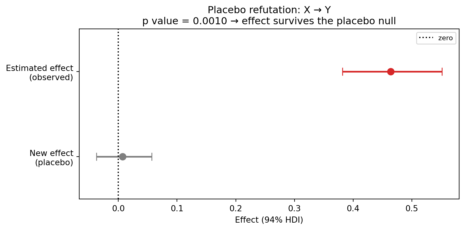

Figure 2: Observed vs. placebo effect. The placebo row sits on zero while the observed row stands well clear of it — the pattern a sound pipeline should produce.

kind="null" shows the full placebo null-predictive distribution with the observed ATE marked. Use it when you want to see the shape of the null the effect is being judged against, rather than a summary interval.

Code

fig, ax = plt.subplots(figsize=(FIG_WIDTH, FIG_HEIGHT))
refutation.plot(ax=ax, kind="null")
plt.tight_layout()
plt.show()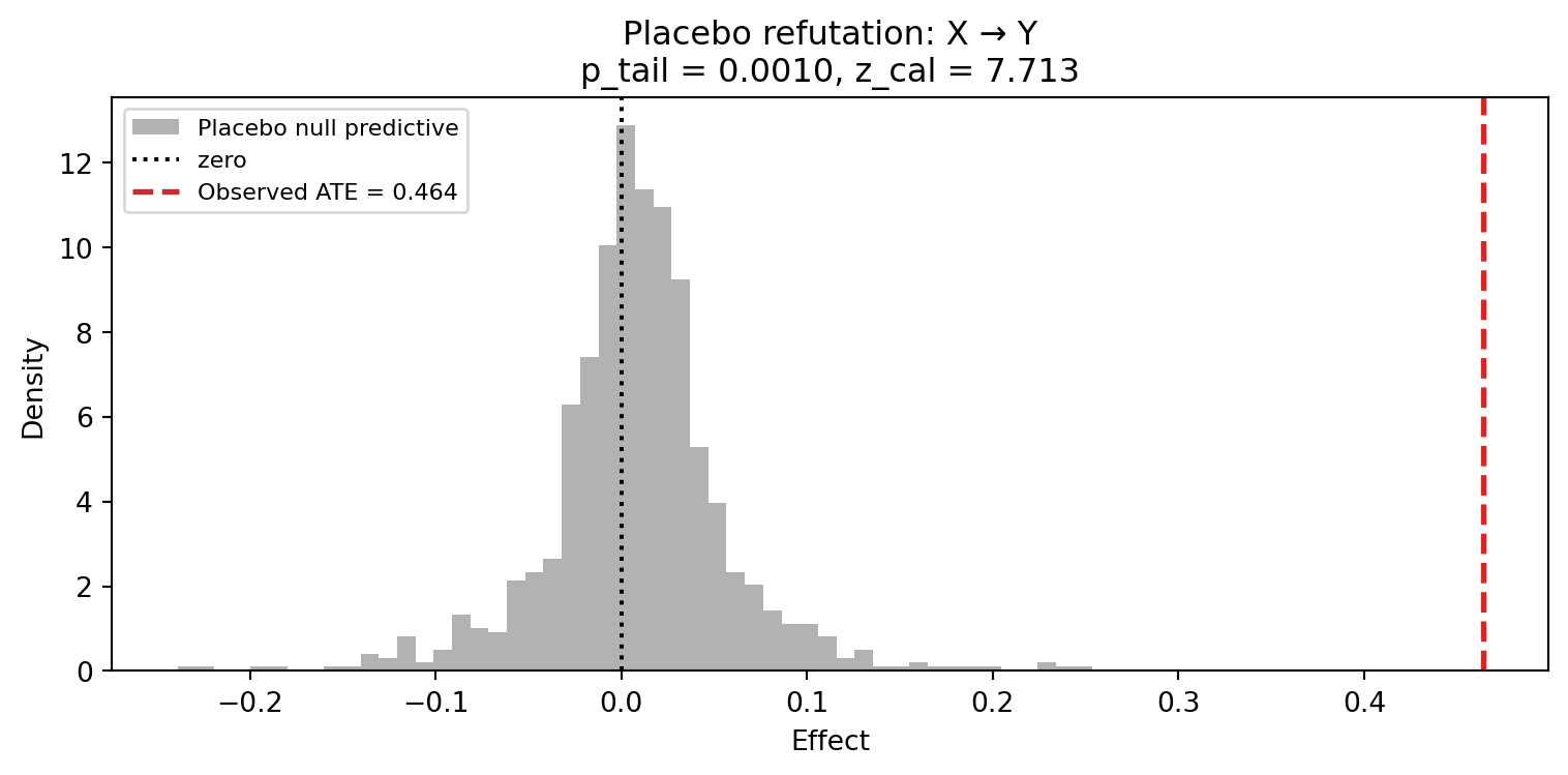

Figure 3: The placebo null-predictive distribution with the observed ATE marked. The observed effect is far outside the range of effects the pipeline produces from permuted treatments.

Read them together: "comparison" is the one to put in a report, "null" is the one to check when a verdict surprises you — a null that is bimodal, skewed, or absurdly wide is telling you something the interval alone hides.

How many permutations?

Cost scales linearly: n_permutations=8 means eight full MCMC re-fits. Precision, though, does not scale with the effect you might expect, because \tau_\text{het} is a variance component estimated from a handful of points. With four folds it is largely prior-dominated, and that prior width propagates straight into the \mu_\text{null} HDI.

refutation_8 = model.refute_placebo(
    "Y",
    "X",
    n_permutations=8,
    sample_kwargs=REFIT,
    random_seed=101,
)

rows = []
for r in (refutation, refutation_8):
    lo, hi = r.mu_null_hdi
    rows.append({
        "folds": r.n_permutations,
        "mu_null": round(r.mu_null, 4),
        "HDI width": round(hi - lo, 4),
        "tau_het": round(r.tau_het, 4),
        "p_tail": round(r.p_tail, 4),
        "passes": r.passes_placebo,
    })
pd.DataFrame(rows).set_index("folds")

NUTS[nutpie]: [beta_Y, sigma_X, beta_X, sigma_Y]
NUTS[nutpie]: [beta_Y, sigma_X, beta_X, sigma_Y]
NUTS[nutpie]: [beta_Y, sigma_X, beta_X, sigma_Y]
NUTS[nutpie]: [beta_Y, sigma_X, beta_X, sigma_Y]
NUTS[nutpie]: [beta_Y, sigma_X, beta_X, sigma_Y]
NUTS[nutpie]: [beta_Y, sigma_X, beta_X, sigma_Y]
NUTS[nutpie]: [beta_Y, sigma_X, beta_X, sigma_Y]
NUTS[nutpie]: [beta_Y, sigma_X, beta_X, sigma_Y]
NUTS[nutpie]: [mu_null, tau_het, z]
Sampling: [theta_new]

	mu_null	HDI width	tau_het	p_tail	passes
folds
4	0.0098	0.1021	0.0352	0.003	True
8	-0.0026	0.0529	0.0202	0.001	True

Doubling the folds roughly halves the width of the placebo-bias interval. That matters in both directions:

A False verdict is trustworthy at four folds. A wide interval that still excludes zero means the bias is real and large.
A True verdict is not. With few folds the inflated interval straddles zero almost automatically, so a genuinely biased pipeline can be waved through. Use eight or more folds before treating a PASS as evidence of soundness.

Four folds is a screening tool: cheap, and adequate to catch gross problems. Eight or more is what you want before publishing a clean bill of health. This is the same small-study problem that Bayesian meta-analysis has studied for years — with only a handful of studies, the heterogeneity parameter is driven by its prior rather than the data, which is exactly why weakly informative scales for it are chosen so carefully (Röver et al. 2021).

When the pipeline fails the test

Permuting the treatment destroys its association with everything, so any coefficient estimated purely from that association collapses to zero. To manufacture an effect from noise you need something that pushes the estimate off zero regardless of the data — and an over-constrained prior does exactly that.

Sign-constrained coefficients are the everyday version of this mistake. Media-mix practitioners routinely impose “spend cannot hurt sales” as a non-negative prior. The constraint is defensible as domain knowledge, but it is not free: a coefficient that cannot be negative cannot average to zero either. Under permutation its posterior piles up just above zero, and the pipeline reports a small positive effect for a treatment it should be blind to.

model_pos = pathmc.model(
    spec,
    data=df,
    priors={"beta_Y": Prior("HalfNormal", sigma=10)},
)
model_pos.fit(random_seed=42, **FIT)

refutation_pos = model_pos.refute_placebo(
    "Y",
    "X",
    n_permutations=8,
    sample_kwargs=REFIT,
    random_seed=101,
)
refutation_pos

NUTS[nutpie]: [beta_Y, sigma_X, beta_X, sigma_Y]

NUTS[nutpie]: [beta_Y, sigma_X, beta_X, sigma_Y]
NUTS[nutpie]: [beta_Y, sigma_X, beta_X, sigma_Y]
NUTS[nutpie]: [beta_Y, sigma_X, beta_X, sigma_Y]
NUTS[nutpie]: [beta_Y, sigma_X, beta_X, sigma_Y]
NUTS[nutpie]: [beta_Y, sigma_X, beta_X, sigma_Y]
NUTS[nutpie]: [beta_Y, sigma_X, beta_X, sigma_Y]
NUTS[nutpie]: [beta_Y, sigma_X, beta_X, sigma_Y]
NUTS[nutpie]: [beta_Y, sigma_X, beta_X, sigma_Y]
NUTS[nutpie]: [mu_null, tau_het, z]
Sampling: [theta_new]

Placebo Refutation: X → Y (α = 0.05)

Placebo test	✗ Fail — the pipeline reports a non-zero effect for a permuted treatment.
Real effect	✓ Survives — the observed effect is too extreme for placebo noise.
Placebo bias μ_null	0.0242 [0.0106, 0.0376]
Structural volatility τ_het	0.0078
Observed ATE	0.4653 [0.3894, 0.5626]
Calibration	z = 17.683, p_tail = 0.0010
Permutations	8

print(f"fold means: {np.round(refutation_pos.fold_means, 4)}")
print(f"all folds positive: {bool(np.all(refutation_pos.fold_means > 0))}")

fold means: [0.0365 0.0174 0.0446 0.032  0.0315 0.0352 0.0153 0.0189]
all folds positive: True

Every fold is positive and the \mu_\text{null} HDI clears zero, so passes_placebo is False. The scatter that made the sound pipeline’s null straddle zero is gone — the constraint rectified it.

Note that effect_survives is still True. The bias is real but tiny next to a 0.5 effect, so the substantive conclusion holds. This is the case for reading the verdict together with the magnitude:

print(f"placebo bias  : {refutation_pos.mu_null:+.4f}")
print(f"observed ATE  : {refutation_pos.observed_ate:+.4f}")
print(
    f"bias as % ATE : {100 * refutation_pos.mu_null / refutation_pos.observed_ate:.1f}%"
)

placebo bias  : +0.0242
observed ATE  : +0.4653
bias as % ATE : 5.2%

passes_placebo has no ROPE

The verdict is a pure interval rule: zero is either inside the HDI or it is not. A negligible bias that happens to be estimated very precisely will fail, as it does here. There is no region of practical equivalence, so always pair the verdict with the ratio above. A bias worth 5% of your effect is a footnote; one worth 100% is the headline.

The same flaw, with the effect it eats

The bias above was harmless because the real effect was large. Shrink the effect until it is the same size as the artifact, and the picture changes completely — a weak true effect (0.05), a smaller sample, and noisier data, with the same non-negative prior:

df_weak = make_data(true_effect=0.05, n=200, noise=1.0, seed=7)

model_weak = pathmc.model(
    spec,
    data=df_weak,
    priors={"beta_Y": Prior("HalfNormal", sigma=10)},
)
model_weak.fit(random_seed=42, **FIT)
model_weak.ate("Y", "X")

NUTS[nutpie]: [beta_Y, sigma_X, beta_X, sigma_Y]

ATE of X on Y

Mean	0.07
94% HDI	[0.00, 0.17]
P(> 0)	1.00
Draws	1000

Methods: .hdi() .prob() .summary() .draws() .by_time() .dataset

Taken at face value that ATE is positive and looks like a finding. The placebo test disagrees:

refutation_weak = model_weak.refute_placebo(
    "Y",
    "X",
    n_permutations=8,
    sample_kwargs=REFIT,
    random_seed=101,
)
refutation_weak

NUTS[nutpie]: [beta_Y, sigma_X, beta_X, sigma_Y]
NUTS[nutpie]: [beta_Y, sigma_X, beta_X, sigma_Y]
NUTS[nutpie]: [beta_Y, sigma_X, beta_X, sigma_Y]
NUTS[nutpie]: [beta_Y, sigma_X, beta_X, sigma_Y]
NUTS[nutpie]: [beta_Y, sigma_X, beta_X, sigma_Y]
NUTS[nutpie]: [beta_Y, sigma_X, beta_X, sigma_Y]
NUTS[nutpie]: [beta_Y, sigma_X, beta_X, sigma_Y]
NUTS[nutpie]: [beta_Y, sigma_X, beta_X, sigma_Y]
NUTS[nutpie]: [mu_null, tau_het, z]
Sampling: [theta_new]

Placebo Refutation: X → Y (α = 0.05)

Placebo test	✗ Fail — the pipeline reports a non-zero effect for a permuted treatment.
Real effect	⚠ Not distinguishable — the observed effect is consistent with placebo noise.
Placebo bias μ_null	0.0908 [0.0400, 0.1366]
Structural volatility τ_het	0.0281
Observed ATE	0.0674 [0.0007, 0.1721]
Calibration	z = -0.298, p_tail = 0.3840
Permutations	8

print(f"placebo bias mu_null : {refutation_weak.mu_null:+.4f}")
print(f"observed ATE         : {refutation_weak.observed_ate:+.4f}")
print(
    f"z_cal / p_tail       : {refutation_weak.z_cal:+.3f} / {refutation_weak.p_tail:.4f}"
)

placebo bias mu_null : +0.0908
observed ATE         : +0.0674
z_cal / p_tail       : -0.298 / 0.3840

Both verdicts now point the same way. passes_placebo is False — the pipeline invents an effect from permuted treatments — and effect_survives is False too, because the observed ATE is no larger than what the pipeline produces from noise. z_cal even comes out negative: the real estimate sits slightly below the placebo null’s center. The apparent finding is the prior talking, not the data.

What to do with a failed placebo test

passes_placebo = False indicts the pipeline, not the dataset. In rough order of how often it is the culprit:

Over-constrained or off-zero priors. Sign constraints and tight informative priors cannot average to zero. Refit with a symmetric prior and see whether the effect holds.
A bounded or heavily skewed outcome. The hierarchical null puts a Gaussian likelihood on the per-fold ATE summaries. For a probability difference near 0 or 1, that is a normal approximation and \mu_\text{null} can drift off zero by construction.
An endogenous treatment. Permuting a regressed variable severs all of its structural links, not just the one to the outcome, so the null describes “treatment decoupled from everything” — a harsher baseline than you may have intended.
Non-convergence in the folds. Each fold is a real MCMC run and can diverge. Inspect fold_sds for an outlier fold that is dominating the pooled null.

Where this sits in the refute suite

The placebo test is one of three complementary checks, and each can pass while another fails:

Check	Question	Fails when
`falsify()`	Is the DAG consistent with the data?	The graph breaks its conditional-independence promises
`sensitivity()`	Could an unmeasured confounder overturn this?	A plausibly weak confounder reaches the tipping point
refute_placebo()	Does the pipeline invent effects?	A permuted treatment still gets a systematic effect

A model can hold a defensible DAG and a robust tipping point while its priors quietly generate effects from noise. Run all three.

Summary

The placebo test severs the treatment-outcome link by permuting the treatment column and re-fitting. A sound pipeline must then report no effect.
The per-permutation posteriors are pooled hierarchically into a systematic bias \mu_\text{null} (should straddle zero) and a structural volatility \tau_\text{het} (the between-shuffle wobble), rather than being collapsed to one point estimate.
passes_placebo judges the machinery: does \mu_\text{null}’s HDI contain zero? effect_survives judges the effect: is p_tail below the significance level when the real ATE is calibrated against the null predictive distribution? They are independent, and both matter.
Use kind="comparison" to report the result and kind="null" to inspect the null’s shape when a verdict surprises you.
Four folds screen; eight or more certify. \tau_\text{het} is a variance component from a handful of points, so a FAIL is informative at four folds while a PASS is not.
Sign-constrained priors are the classic way to fail. A coefficient that cannot go negative cannot average to zero under permutation.
The verdict carries no region of practical equivalence, so read it next to the bias-to-effect ratio: the same flaw is a footnote against a large effect and fatal against a weak one.

Reflection

Which priors in your own model are constrained by sign or centered away from zero? What would the placebo bias be if the treatment carried no information at all?
Your effect passes at four folds. What would you need to see before reporting that as evidence the pipeline is unbiased?
Suppose passes_placebo fails with a bias worth 3% of your estimated effect. Do you report the effect, the failure, or both — and what would change your mind?

References

Bugaev, Anton, and Carlos Trujillo. n.d. “Bayesian Design Analysis for Time-Series Quasi-Experiments: A Placebo-Calibrated Framework.” Unpublished manuscript.

Röver, Christian, Ralf Bender, Sofia Dias, et al. 2021. “On Weakly Informative Prior Distributions for the Heterogeneity Parameter in Bayesian Random-Effects Meta-Analysis.” Research Synthesis Methods 12 (4): 448–74. https://doi.org/10.1002/jrsm.1475.

Sharma, Amit, and Emre Kiciman. 2020. DoWhy: An End-to-End Library for Causal Inference. https://doi.org/10.48550/arXiv.2011.04216.