Panel Data Models

From cross-sectional snapshots to temporal dynamics — compare cross-sectional and panel DAGs, model AR(1) persistence with lag(Y), and run time-forward interventions with adstock transforms.

Author

Benjamin Vincent

You want to know if promotional spending causes higher store revenue. You collect data. But whether your data is a snapshot of many stores at one point in time or the same stores tracked over many weeks fundamentally changes the DAG you draw — and the causal story you can tell.

Cross-sectional data captures associations at a single moment. Panel data adds temporal ordering, which introduces new causal paths (carry-over effects, lagged dependencies) and new tools for identification. The same business question leads to different DAGs, different models, and often different conclusions.

This notebook builds panel models of increasing complexity:

Cross-sectional vs panel DAGs — how temporal structure changes the causal graph, and what you miss without it
AR(1) persistence — modelling outcome momentum with lag(Y), the long-run multiplier, and ramp-up dynamics
Transforms in panel — adstock and saturation with time-forward interventions

Setup

import numpy as np
import pandas as pd
import matplotlib.pyplot as plt
import arviz as az
import pymc as pm
import pathmc

FIG_WIDTH = 8
FIG_HEIGHT = 4

COLOR_PROMO = "#2171b5"
COLOR_REVENUE = "#31a354"
COLOR_TRAFFIC = "#e6550d"
COLOR_CONTEMP = "#756bb1"
COLOR_LAG = "#e7298a"
COLOR_EFFECT = "#2171b5"
COLOR_BOOST = "#31a354"
COLOR_THEORY = "#756bb1"

rng = np.random.default_rng(42)

1. Cross-sectional vs panel DAGs

The scenario

A retail chain asks: does promotional spending increase store revenue?

They have data from 500 stores collected during a single week. Each store reported its promotional budget, foot traffic count, and total revenue.

But stores with higher foot traffic tend to spend more on promotions and generate more revenue — not because promotions cause traffic, but because busy stores have bigger budgets and more customers. If we don’t account for foot traffic, we’ll confuse the effect of promotions with the effect of being a high-traffic store.

The cross-sectional DAG

Figure 1: Cross-sectional DAG: foot_traffic confounds the promo → revenue relationship. All edges represent contemporaneous associations at a single point in time.

Three things to read from this DAG:

foot_traffic → promo: stores with more foot traffic invest more in promotions (confounding path)
foot_traffic → revenue: more traffic means more sales regardless of promotions (confounding path)
promo → revenue: the causal path we want to isolate

What a cross-sectional DAG assumes about time

Cross-sectional DAGs treat all relationships as happening simultaneously. The arrow promo → revenue doesn’t say “promo at time t causes revenue at time t” — it says “differences in promo correspond to differences in revenue, and we assume the causal direction runs from promo to revenue.”

This is reasonable when effects are near-instantaneous relative to the measurement interval. But it cannot represent carry-over, delay, or accumulation — effects that unfold over time.

Simulate and fit the cross-sectional model

n_cs = 500

TRUE_CONFOUND = 0.6
TRUE_B_PROMO = 0.5
TRUE_B_TRAFFIC_CS = 0.8

foot_traffic = rng.normal(0, 1, size=n_cs)
promo = 2 + TRUE_CONFOUND * foot_traffic + rng.normal(0, 0.5, size=n_cs)
revenue = (
    5
    + TRUE_B_PROMO * promo
    + TRUE_B_TRAFFIC_CS * foot_traffic
    + rng.normal(0, 1, size=n_cs)
)

df_cs = pd.DataFrame({
    "foot_traffic": foot_traffic,
    "promo": promo,
    "revenue": revenue,
})

print(f"N = {n_cs}")
print(f"True causal effect of promo on revenue: {TRUE_B_PROMO}")
df_cs.describe().round(2)

N = 500
True causal effect of promo on revenue: 0.5

	foot_traffic	promo	revenue
count	500.00	500.00	500.00
mean	-0.01	1.97	5.97
std	0.96	0.77	1.52
min	-2.57	-0.65	1.15
25%	-0.67	1.46	5.02
50%	0.00	2.00	5.92
75%	0.59	2.50	7.01
max	2.91	4.14	10.67

The spec encodes the full confounded DAG. The equation for revenue includes both promo and foot_traffic, adjusting for the confounder.

spec_cs = """
promo ~ foot_traffic
revenue ~ b_promo*promo + foot_traffic
"""

model_cs = pathmc.model(spec_cs, data=df_cs)
model_cs.graph()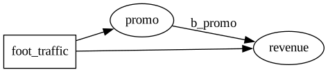

idata_cs = model_cs.fit(draws=500, tune=500, chains=2, random_seed=42)

NUTS[nutpie]: [beta_revenue, sigma_promo, beta_promo, sigma_revenue]

model_cs.effects_summary()

	mean	sd	hdi_3%	hdi_97%
name
b_promo	0.425964	0.091139	0.271312	0.612291

The labeled coefficient b_promo should be close to the true value of 0.5. The do() operator confirms — setting promo regardless of foot traffic isolates the causal effect:

ate_cs = model_cs.ate("revenue", "promo", values=(1.0, 3.0))
ate_cs

ATE of promo on revenue

Mean	0.85
94% HDI	[0.54, 1.22]
P(> 0)	1.00
Draws	1000

Methods: .hdi() .prob() .summary() .draws() .by_time() .dataset

The expected causal effect for a 2-unit increase in promo is TRUE_B_PROMO × 2 = 1.0.

This works, but it assumes the effect is instantaneous — no carry-over, no temporal dynamics. If promotions take time to affect revenue, the cross-sectional estimate captures only part of the story.

Adding time: the panel DAG

Suppose internal research reveals that promotions have two effects:

An immediate effect: some customers respond this week
A carry-over effect: some customers see the promotion this week but buy next week

The cross-sectional model cannot distinguish these. Panel data — the same stores observed over many weeks — lets us model both by introducing lagged variables into the DAG.

Figure 2: Panel DAG showing two time slices. The contemporaneous edge (promo_t → revenue_t) captures the immediate effect. The lagged edge (promo_{t−1} → revenue_t, dashed) captures carry-over.

Compare this to the cross-sectional DAG in Figure 1. Two critical differences:

A new edge appears: promo_{t-1} → revenue_t. This carry-over path doesn’t exist in a snapshot because there’s no “previous week.”
Temporal ordering aids identification: because causes must precede effects, the direction of the lagged edge is unambiguous — last week’s promo cannot be caused by this week’s revenue.

New edges from temporal ordering

Panel DAGs can have edges that are impossible in a cross-sectional DAG. Any lagged relationship — X_{t-k} \to Y_t — represents a causal mechanism that unfolds over time. These edges expand the set of causal paths and change the total effect of an intervention.

Simulate and fit the panel model

n_stores = 8
n_weeks = 30
store_names = [f"S{i + 1}" for i in range(n_stores)]

TRUE_CONTEMP = 0.30
TRUE_LAG = 0.25
TRUE_B_TRAFFIC_PANEL = 0.6

store_ft_bases = {s: rng.normal(0, 0.5) for s in store_names}
store_rev_bases = {s: rng.normal(5, 1.0) for s in store_names}

rows = []
for store in store_names:
    prev_promo = 2.0
    for week in range(1, n_weeks + 1):
        ft = store_ft_bases[store] + rng.normal(0, 0.3)
        p = 2 + TRUE_CONFOUND * ft + rng.normal(0, 0.5)
        r = (
            store_rev_bases[store]
            + TRUE_CONTEMP * p
            + TRUE_LAG * prev_promo
            + TRUE_B_TRAFFIC_PANEL * ft
            + rng.normal(0, 1)
        )
        rows.append({
            "store": store,
            "week": week,
            "foot_traffic": ft,
            "promo": p,
            "revenue": r,
        })
        prev_promo = p

df_panel = pd.DataFrame(rows)
print(f"Panel: {n_stores} stores × {n_weeks} weeks = {len(df_panel)} rows")
print(f"True contemporaneous effect: {TRUE_CONTEMP}")
print(f"True lagged effect:          {TRUE_LAG}")
print(f"True total effect:           {TRUE_CONTEMP + TRUE_LAG}")

Panel: 8 stores × 30 weeks = 240 rows
True contemporaneous effect: 0.3
True lagged effect:          0.25
True total effect:           0.55

The lag(promo) term tells pathmc to include last week’s promo as a predictor. The panel argument identifies units and time; pooling="partial" adds random intercepts per store.

spec_panel = """
promo ~ foot_traffic
revenue ~ b_contemp*promo + b_lag*lag(promo) + foot_traffic
"""

model_panel = pathmc.model(
    spec_panel,
    data=df_panel,
    panel={"unit": "store", "time": "week"},
    pooling="partial",
)
model_panel.graph()

/Users/benjamv/git/copilot-worktrees/pathmc/drbenvincent-literate-couscous/pathmc/_model.py:165: UserWarning: 
==============================================================================
PARTIAL POOLING WITH REDUNDANT INTERCEPT
==============================================================================

Your model uses pooling='partial' (random intercepts) but the following
equations include a formula intercept: 'promo', 'revenue'.

This creates a NON-IDENTIFIABLE parameterization:
  • beta[Intercept] (fixed global intercept)
  • mu_alpha (mean of random intercepts)
Only their sum is identified by the data. This causes sampling divergences.

SOLUTION: Remove the intercept from your formula(s):

  promo ~ 0 + foot_traffic
  revenue ~ 0 + b_contemp*promo + b_lag*lag(promo) + foot_traffic

The hierarchical mean mu_alpha will serve as the effective intercept.
==============================================================================

  self._compile()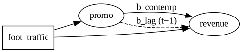

idata_panel = model_panel.fit(draws=500, tune=500, chains=2, random_seed=42)

NUTS[nutpie]: [sigma_promo, sigma_alpha_revenue, mu_alpha_revenue, alpha_revenue, sigma_alpha_promo, mu_alpha_promo, alpha_promo, beta_revenue, beta_promo, carry_innovations_promo, sigma_revenue]

model_panel.effects_summary()

	mean	sd	hdi_3%	hdi_97%
name
b_contemp	0.188710	0.111635	-0.005537	0.403733
b_lag	0.446661	0.097026	0.266532	0.634403

Reading the decomposed effect

The panel model recovers two separate coefficients:

b_contemp ≈ 0.30: the immediate effect of this week’s promo
b_lag ≈ 0.25: the carry-over effect of last week’s promo
Total ≈ 0.55: the full short-run impact of a sustained promotion

A cross-sectional analysis would estimate a single blended number — unable to distinguish immediate response from carry-over.

Code

contemp_draws = (
    idata_panel
    .posterior["beta_revenue"]
    .sel(revenue_predictors="promo")
    .values.flatten()
)
lag_draws = (
    idata_panel
    .posterior["beta_revenue"]
    .sel(revenue_predictors="lag(promo)")
    .values.flatten()
)
total_draws = contemp_draws + lag_draws

fig, axes = plt.subplots(1, 3, figsize=(FIG_WIDTH, FIG_HEIGHT))

for ax, draws, color, label, true_val in [
    (
        axes[0],
        contemp_draws,
        COLOR_CONTEMP,
        "Contemporaneous\n(b_contemp)",
        TRUE_CONTEMP,
    ),
    (axes[1], lag_draws, COLOR_LAG, "Carry-over\n(b_lag)", TRUE_LAG),
    (
        axes[2],
        total_draws,
        COLOR_PROMO,
        "Total\n(b_contemp + b_lag)",
        TRUE_CONTEMP + TRUE_LAG,
    ),
]:
    x_kde, y_kde, _ = az.kde(draws)
    ax.plot(x_kde, y_kde, color=color, lw=2)
    ax.fill_between(x_kde, y_kde, alpha=0.3, color=color)
    ax.axvline(draws.mean(), color=color, ls="--", lw=1.5, alpha=0.7)
    ax.axvline(true_val, color="black", ls="--", lw=1.5, alpha=0.5)
    ax.set_xlabel(label)
    ax.set_ylabel("Density" if ax == axes[0] else "")

plt.tight_layout()
plt.show()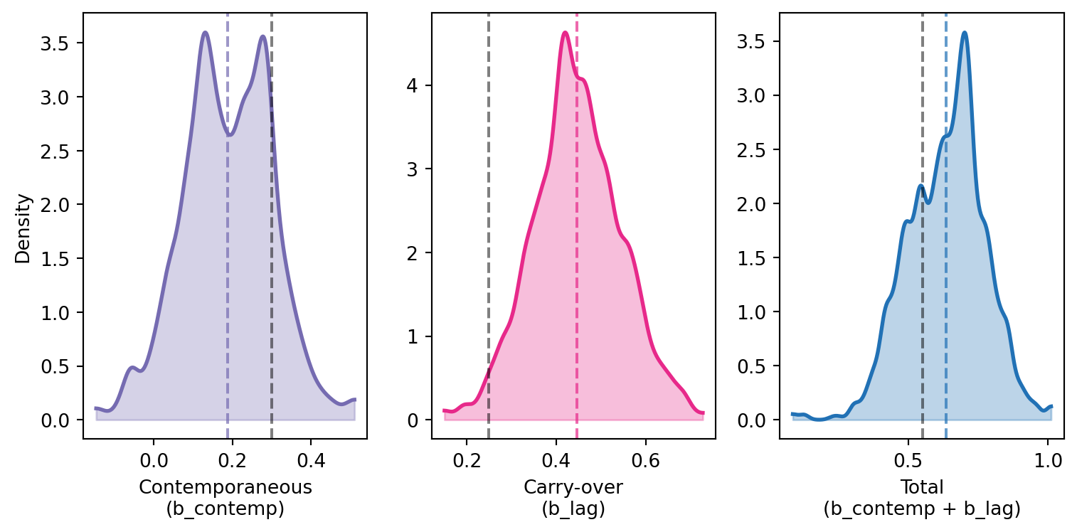

Figure 3: Posterior distributions of the contemporaneous and lagged promo effects from the panel model. Black dashed lines mark the true DGP values.

Time-forward do() propagates the intervention through lagged variables — from the second step onward, lag(promo) picks up the intervened value:

ate_panel = model_panel.ate(
    "revenue",
    "promo",
    values=(1.0, 3.0),
    simulate_over="time",
)

print(f"Steady-state expected: {(TRUE_CONTEMP + TRUE_LAG) * 2:.3f}")
ate_panel

Steady-state expected: 1.100

ATE of promo on revenue

Mean	0.00
94% HDI	[0.00, 0.00]
P(> 0)	0.00
Draws	1000

Methods: .hdi() .prob() .summary() .draws() .by_time() .dataset

What happens if you ignore the lags?

To make the comparison concrete, let’s fit the panel data without the lag term — pretending the data has a cross-sectional structure.

spec_no_lag = """
promo ~ foot_traffic
revenue ~ b_naive*promo + foot_traffic
"""

model_no_lag = pathmc.model(
    spec_no_lag,
    data=df_panel,
    panel={"unit": "store", "time": "week"},
    pooling="partial",
)
idata_no_lag = model_no_lag.fit(draws=500, tune=500, chains=2, random_seed=42)

/Users/benjamv/git/copilot-worktrees/pathmc/drbenvincent-literate-couscous/pathmc/_model.py:165: UserWarning: 
==============================================================================
PARTIAL POOLING WITH REDUNDANT INTERCEPT
==============================================================================

Your model uses pooling='partial' (random intercepts) but the following
equations include a formula intercept: 'promo', 'revenue'.

This creates a NON-IDENTIFIABLE parameterization:
  • beta[Intercept] (fixed global intercept)
  • mu_alpha (mean of random intercepts)
Only their sum is identified by the data. This causes sampling divergences.

SOLUTION: Remove the intercept from your formula(s):

  promo ~ 0 + foot_traffic
  revenue ~ 0 + b_naive*promo + foot_traffic

The hierarchical mean mu_alpha will serve as the effective intercept.
==============================================================================

  self._compile()
NUTS[nutpie]: [sigma_alpha_revenue, mu_alpha_revenue, alpha_revenue, beta_revenue, sigma_promo, sigma_alpha_promo, mu_alpha_promo, alpha_promo, beta_promo, sigma_revenue]

Code

naive_draws = (
    idata_no_lag
    .posterior["beta_revenue"]
    .sel(revenue_predictors="promo")
    .values.flatten()
)

fig, ax = plt.subplots(figsize=(FIG_WIDTH, FIG_HEIGHT * 0.8))

for draws, color, label in [
    (naive_draws, COLOR_CONTEMP, "Naive (no lag)"),
    (total_draws, COLOR_PROMO, "Panel (contemp + lag)"),
]:
    x_kde, y_kde, _ = az.kde(draws)
    ax.plot(x_kde, y_kde, color=color, lw=2, label=label)
    ax.fill_between(x_kde, y_kde, alpha=0.25, color=color)
    ax.axvline(draws.mean(), color=color, ls="--", alpha=0.7, lw=1)

ax.axvline(
    TRUE_CONTEMP + TRUE_LAG,
    color="black",
    ls="--",
    lw=1.5,
    alpha=0.5,
    label=f"True total ({TRUE_CONTEMP + TRUE_LAG})",
)
ax.set_xlabel("Effect of promo on revenue")
ax.set_ylabel("Density")
ax.legend()
plt.tight_layout()
plt.show()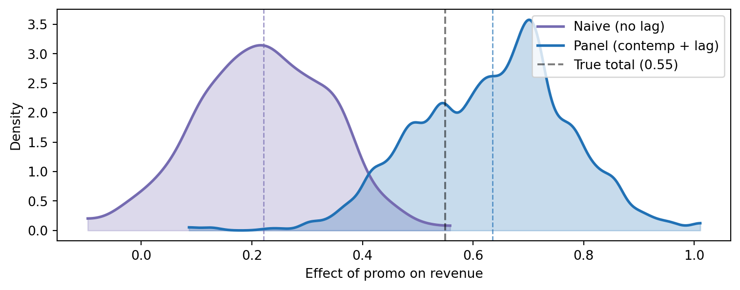

Figure 4: Naive model without lag term (purple) vs panel model total effect (blue). The naive model underestimates the total effect by missing the carry-over path. Black dashed line: true total effect.

The naive model captures only the contemporaneous effect. The carry-over path promo_{t-1} → revenue_t is invisible to it, so roughly half the total effect is missed.

Cross-sectional vs panel: a comparison

Feature	Cross-Sectional	Panel
Data structure	N units × 1 time point	N units × T time points
DAG edges	All contemporaneous	Contemporaneous + lagged
Temporal effects	Cannot decompose	Separate contemporaneous vs carry-over
Identification	Adjust via observed confounders	+ temporal ordering provides unambiguous causal direction
Pooling	Not applicable	Partial pooling borrows strength across units
do() operator	Single-step propagation	Time-forward simulation resolves lags dynamically

2. AR(1) persistence

The previous section showed how an input can have lagged effects on an outcome. But what about the outcome itself? Many business quantities — engagement, brand equity, customer satisfaction — are persistent: today’s value depends on yesterday’s.

An AR(1) model captures this by including the lagged outcome as a predictor:

Y_t = \beta_0 + \beta_X \cdot X_t + \rho \cdot Y_{t-1} + \varepsilon_t

The coefficient \rho controls how much of the previous period’s value carries forward. When 0 < \rho < 1, the system is stationary: shocks accumulate but eventually decay. The long-run multiplier of X is \beta_X / (1 - \rho) — often much larger than the immediate effect \beta_X alone.

The autoregressive DAG

Figure 5: Autoregressive DAG. X has a direct contemporaneous effect on Y, and Y feeds back into itself through a one-period lag.

A one-unit increase in X at time t affects Y_t directly (by \beta_X), but also Y_{t+1} (through \rho \cdot Y_t), Y_{t+2} (through \rho^2), and so on. The total long-run effect is the geometric series \beta_X \sum_{k=0}^{\infty} \rho^k = \beta_X / (1 - \rho).

Immediate vs long-run effects

With \beta_X = 0.4 and \rho = 0.6, each unit of promotion spend lifts engagement by 0.4 this week — but the cumulative long-run effect is 0.4 / (1 - 0.6) = 1.0. The AR(1) dynamics amplify the immediate effect by a factor of 1 / (1 - \rho) = 2.5\times.

Simulate and fit

n_weeks_ar = 50
true_intercept = 2.0
true_beta_x = 0.4
true_rho = 0.6
true_sigma = 0.5

rows_ar = []
y = 0.0
for week in range(1, n_weeks_ar + 1):
    promo_val = rng.uniform(0, 10)
    y = (
        true_intercept
        + true_beta_x * promo_val
        + true_rho * y
        + rng.normal(scale=true_sigma)
    )
    rows_ar.append({
        "country": "national",
        "week": week,
        "promotion": promo_val,
        "engagement": y,
    })

df_ar = pd.DataFrame(rows_ar)

true_longrun = true_beta_x / (1 - true_rho)
print(f"True immediate effect: β_x = {true_beta_x}")
print(f"True persistence:      ρ   = {true_rho}")
print(f"True long-run effect:  β_x / (1 − ρ) = {true_longrun}")

True immediate effect: β_x = 0.4
True persistence:      ρ   = 0.6
True long-run effect:  β_x / (1 − ρ) = 1.0

Code

fig, ax = plt.subplots(figsize=(FIG_WIDTH, FIG_HEIGHT))
ax.plot(df_ar["week"], df_ar["engagement"], color=COLOR_EFFECT, lw=1.5)
ax.scatter(df_ar["week"], df_ar["engagement"], color=COLOR_EFFECT, s=15, zorder=3)
ax.set_xlabel("Week")
ax.set_ylabel("Engagement")
plt.tight_layout()
plt.show()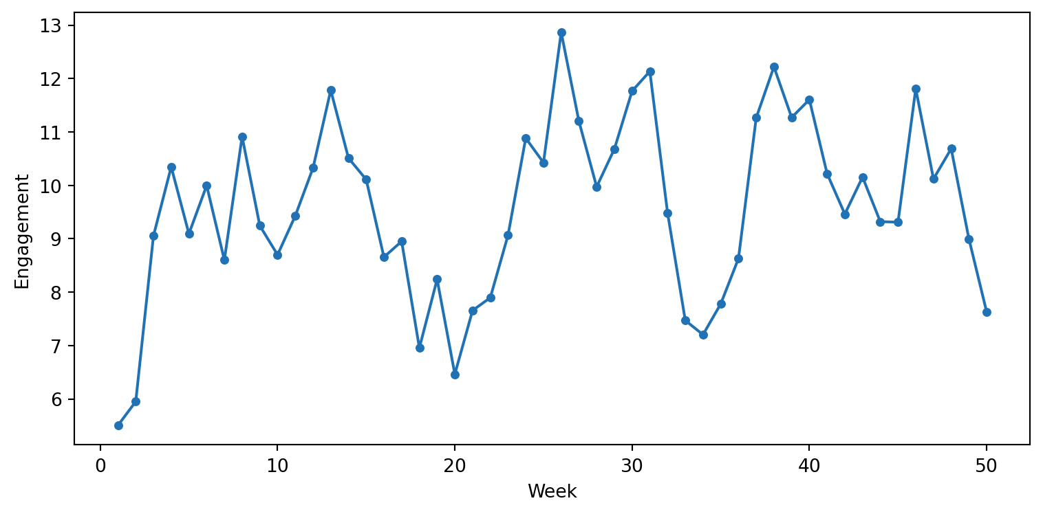

Figure 6: Weekly engagement over 50 weeks. The series is persistent — high values tend to follow high values — reflecting the AR(1) structure.

The lag(engagement) term tells pathmc to include the previous period’s outcome as a predictor:

spec_ar = "engagement ~ b_x*promotion + rho*lag(engagement)"

model_ar = pathmc.model(
    spec_ar,
    data=df_ar,
    panel={"unit": "country", "time": "week"},
)

idata_ar = model_ar.fit(draws=200, tune=200, chains=4, random_seed=42)

NUTS[nutpie]: [sigma_engagement, beta_engagement, carry_innovations_engagement]

model_ar.effects_summary()

	mean	sd	hdi_3%	hdi_97%
name
b_x	0.373871	0.034005	0.308365	0.433238
rho	0.698864	0.055312	0.591866	0.797471

The long-run multiplier

The long-run effect is a nonlinear function of two parameters (\beta_X / (1 - \rho)), so we compute it from the joint posterior to get the full uncertainty.

Code

b_x_draws = (
    idata_ar
    .posterior["beta_engagement"]
    .sel(engagement_predictors="promotion")
    .values.flatten()
)
rho_draws = (
    idata_ar
    .posterior["beta_engagement"]
    .sel(engagement_predictors="lag(engagement)")
    .values.flatten()
)
longrun_draws = b_x_draws / (1 - rho_draws)

fig, ax = plt.subplots(figsize=(FIG_WIDTH, FIG_HEIGHT))
x_kde, y_kde, _ = az.kde(longrun_draws)
ax.plot(x_kde, y_kde, color=COLOR_EFFECT, lw=2, label="Posterior")
ax.fill_between(x_kde, y_kde, alpha=0.25, color=COLOR_EFFECT)
ax.axvline(
    true_longrun, color=COLOR_THEORY, ls="--", lw=2, label=f"True = {true_longrun:.1f}"
)
ax.axvline(
    true_beta_x,
    color=COLOR_TRAFFIC,
    ls=":",
    lw=2,
    label=f"Immediate only = {true_beta_x}",
)
ax.set_xlabel("Long-run multiplier: β_x / (1 − ρ)")
ax.set_ylabel("Density")
ax.legend()
plt.tight_layout()
plt.show()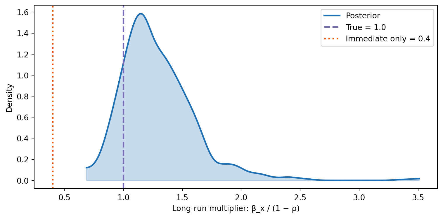

Figure 7: Posterior distribution of the long-run multiplier β_x / (1 − ρ). The immediate effect alone (orange dotted) substantially understates the total impact.

Ramp-up dynamics

What happens to engagement over time when we set promotion to a constant level? With an AR(1) model, engagement doesn’t jump to the long-run level instantly — it ramps up over several periods as the lagged effect accumulates.

r_lo = model_ar.do(set={"promotion": 2.0}, simulate_over="time", kind="mean")
r_hi = model_ar.do(set={"promotion": 8.0}, simulate_over="time", kind="mean")
contrast_ar = r_hi - r_lo

Code

fig, ax = plt.subplots(figsize=(FIG_WIDTH, FIG_HEIGHT))

weeks_ar = np.arange(1, n_weeks_ar + 1)
engagement_by_time = contrast_ar.by_time("engagement")

ax.plot(
    weeks_ar,
    engagement_by_time.mean(axis=1),
    color=COLOR_EFFECT,
    lw=2,
    label="Posterior mean",
)
hdi_1 = az.hdi(engagement_by_time.T, prob=0.94, axis=0)
ax.fill_between(
    weeks_ar, hdi_1[:, 0], hdi_1[:, 1], alpha=0.15, color=COLOR_EFFECT, label="94% HDI"
)

delta_x = 8.0 - 2.0
ax.axhline(
    true_beta_x * delta_x,
    color=COLOR_TRAFFIC,
    ls=":",
    lw=1.5,
    label=f"Immediate effect = {true_beta_x * delta_x:.1f}",
)
ax.axhline(
    true_longrun * delta_x,
    color=COLOR_THEORY,
    ls="--",
    lw=1.5,
    label=f"Long-run effect = {true_longrun * delta_x:.1f}",
)

ax.set_xlabel("Week")
ax.set_ylabel("Incremental engagement (promo 8 − promo 2)")
ax.legend(fontsize=8)
ax.axhline(0, color="black", ls=":", alpha=0.3)
plt.tight_layout()
plt.show()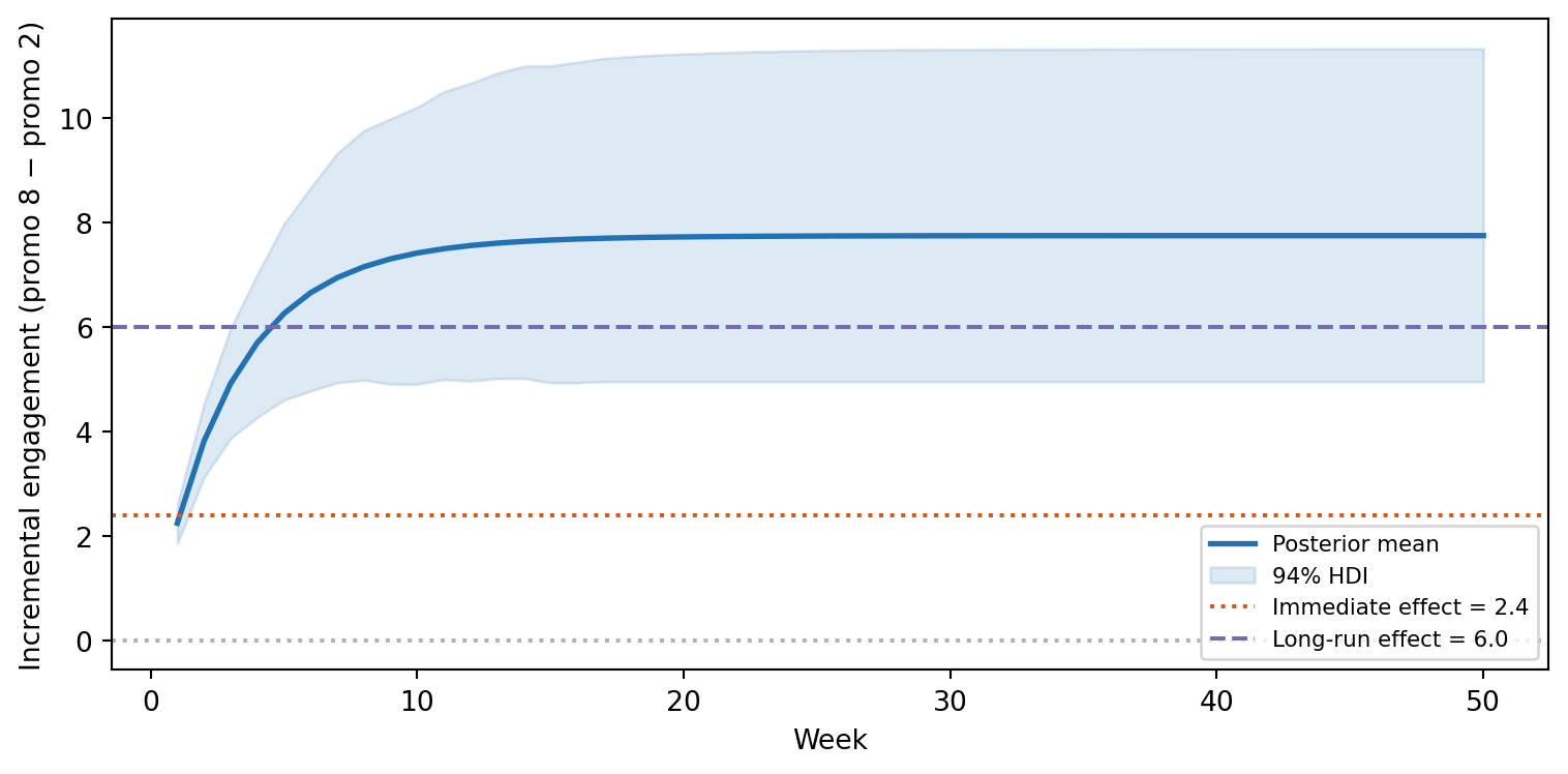

Figure 8: Time profile of the causal effect of increasing promotion from 2 to 8 units. The effect ramps up over ~10 weeks as AR(1) dynamics accumulate, then converges to the long-run steady state.

The ramp-up shape is characteristic of AR(1) dynamics:

Week 1: the effect equals the immediate impact \beta_X \cdot \Delta X
Weeks 2–10: each period adds \rho times the previous period’s effect
Week 10+: the effect converges to the long-run level \frac{\beta_X}{1 - \rho} \cdot \Delta X

The half-life — how many periods to reach half the long-run effect — is \log(0.5) / \log(\rho) \approx 1.4 weeks for \rho = 0.6.

3. Transforms in panel models

In marketing analytics, carry-over is typically modeled with adstock transforms rather than raw lag terms. Adstock combines geometric decay with saturation curves, capturing two phenomena at once: the carry-over of past spend into future effects, and diminishing returns at high spend levels.

pathmc compiles these transforms using pytensor.scan, encoding the full temporal recurrence in the generative model. When you call do(simulate_over="time"), the scan propagates the intervention forward through time — no separate simulation engine needed.

Simulate a multi-channel panel

We simulate a 2-channel MMM panel with adstock carry-over, logistic saturation, and region-specific intercepts.

regions = ["North", "South", "East", "West"]
n_weeks_mmm = 40
true_intercepts = {"North": 50, "South": 60, "East": 45, "West": 55}
true_decay_tv = 0.7
true_decay_dig = 0.7
true_lam_tv = 0.03
true_lam_dig = 0.02
true_b_tv = 25.0
true_b_dig = 30.0

rows_mmm = []
for region in regions:
    adstocked_tv = 0.0
    adstocked_dig = 0.0
    for week in range(1, n_weeks_mmm + 1):
        tv = rng.uniform(10, 50)
        digital = rng.uniform(5, 30)
        adstocked_tv = tv + true_decay_tv * adstocked_tv
        adstocked_dig = digital + true_decay_dig * adstocked_dig
        sat_tv = 1 - np.exp(-true_lam_tv * adstocked_tv)
        sat_dig = 1 - np.exp(-true_lam_dig * adstocked_dig)
        sales = (
            true_intercepts[region]
            + true_b_tv * sat_tv
            + true_b_dig * sat_dig
            + 0.1 * week
            + rng.normal(scale=1.5)
        )
        rows_mmm.append({
            "region": region,
            "week": week,
            "tv": tv,
            "digital": digital,
            "trend": week,
            "sales": sales,
        })

df_mmm = pd.DataFrame(rows_mmm)
print(f"Panel: {len(regions)} regions × {n_weeks_mmm} weeks = {len(df_mmm)} rows")
df_mmm.head()

Panel: 4 regions × 40 weeks = 160 rows

	region	week	tv	digital	trend	sales
0	North	1	49.487453	6.122008	1	74.466792
1	North	2	12.874487	19.803321	2	80.374423
2	North	3	24.368176	5.273368	3	82.811692
3	North	4	49.649785	11.440436	4	85.176618
4	North	5	14.957036	18.881390	5	89.961273

Fit the model

spec_mmm = """
sales ~ b_tv*logistic_saturation(adstock(tv, decay=theta_tv), lam=lam_tv)
      + b_dig*logistic_saturation(adstock(digital, decay=theta_dig), lam=lam_dig)
      + trend
"""

model_mmm = pathmc.model(
    spec_mmm,
    data=df_mmm,
    panel={"unit": "region", "time": "week"},
    pooling="partial",
)
model_mmm.equations()

/Users/benjamv/git/copilot-worktrees/pathmc/drbenvincent-literate-couscous/pathmc/_model.py:165: UserWarning: 
==============================================================================
PARTIAL POOLING WITH REDUNDANT INTERCEPT
==============================================================================

Your model uses pooling='partial' (random intercepts) but the following
equations include a formula intercept: 'sales'.

This creates a NON-IDENTIFIABLE parameterization:
  • beta[Intercept] (fixed global intercept)
  • mu_alpha (mean of random intercepts)
Only their sum is identified by the data. This causes sampling divergences.

SOLUTION: Remove the intercept from your formula(s):

  sales ~ 0 + b_tv*logistic_saturation(adstock(tv, decay=theta_tv), lam=lam_tv) + b_dig*logistic_saturation(adstock(digital, decay=theta_dig), lam=lam_dig) + trend

The hierarchical mean mu_alpha will serve as the effective intercept.
==============================================================================

  self._compile()

\begin{aligned} \beta_{sales} &\sim \text{Normal}(mu=0,\, sigma=10) \\ \sigma_{sales} &\sim \text{HalfNormal}(sigma=1) \\ \mu_{alpha,sales} &\sim \text{Normal}(mu=0,\, sigma=10) \\ \sigma_{alpha,sales} &\sim \text{HalfNormal}(sigma=1) \\ \alpha_{sales} &\sim \text{Normal}(mu\_alpha,\, sigma\_alpha) \\ \theta_{tv} &\sim \text{Beta}(alpha=2,\, beta=2) \\ \lambda_{tv} &\sim \text{HalfNormal}(sigma=1) \\ \theta_{dig} &\sim \text{Beta}(alpha=2,\, beta=2) \\ \lambda_{dig} &\sim \text{HalfNormal}(sigma=1) \\[6pt] \mu_{sales} &= \beta_{0,\,sales} \\ &\quad + b_{tv} \cdot \operatorname{logistic\_saturation}(\operatorname{adstock}(\mathrm{tv},\, \theta_{tv}),\, \lambda_{tv}) \\ &\quad + b_{dig} \cdot \operatorname{logistic\_saturation}(\operatorname{adstock}(\mathrm{digital},\, \theta_{dig}),\, \lambda_{dig}) \\ &\quad + \mathrm{trend} \\ \mathrm{sales} &\sim \text{Normal}(\mu_{sales},\, \sigma_{sales}) \end{aligned}

model_mmm.fit(draws=500, tune=500, chains=4, random_seed=42)

NUTS[nutpie]: [sigma_alpha_sales, mu_alpha_sales, alpha_sales, lam_dig, theta_dig, lam_tv, theta_tv, beta_sales, sigma_sales]

A temporary intervention

We increase digital spend by 15% for a fixed 10-week window (weeks 11–20), leaving TV unchanged. Because digital has adstock carry-over, the effect on sales will ramp up during the boost as the adstock stock accumulates, and ramp down after the boost ends as the stock decays.

mean_digital = df_mmm["digital"].mean()
boost_fraction = 0.15
boost_start, boost_end = 10, 20

digital_baseline = np.full(n_weeks_mmm, mean_digital)
digital_scenario = digital_baseline.copy()
digital_scenario[boost_start:boost_end] = mean_digital * (1 + boost_fraction)

Code

fig, ax = plt.subplots(figsize=(FIG_WIDTH, FIG_HEIGHT * 0.7))
weeks_mmm = np.arange(1, n_weeks_mmm + 1)
ax.plot(weeks_mmm, digital_baseline, color="gray", ls="--", label="Baseline digital")
ax.plot(
    weeks_mmm,
    digital_scenario,
    color=COLOR_BOOST,
    lw=2,
    label="Scenario digital (+15%)",
)
ax.axvspan(
    boost_start + 1, boost_end, alpha=0.1, color=COLOR_BOOST, label="Boost window"
)
ax.set_xlabel("Week")
ax.set_ylabel("Digital spend")
ax.legend(loc="upper right")
plt.tight_layout()
plt.show()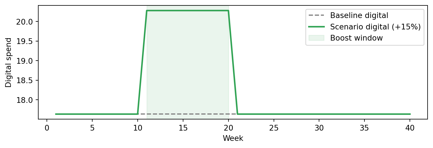

Figure 9: Intervention design: digital spend increased by 15% during weeks 11–20 (shaded), then returns to baseline.

result_baseline = model_mmm.do(
    set={"digital": digital_baseline},
    simulate_over="time",
)
result_scenario = model_mmm.do(
    set={"digital": digital_scenario},
    simulate_over="time",
)
contrast_mmm = result_scenario - result_baseline

Code

fig, ax = plt.subplots(figsize=(FIG_WIDTH, FIG_HEIGHT))

sales_by_time = contrast_mmm.by_time("sales")

ax.plot(
    weeks_mmm,
    sales_by_time.mean(axis=1),
    color=COLOR_EFFECT,
    lw=2,
    label="Posterior mean",
)
hdi_2 = az.hdi(sales_by_time.T, prob=0.94, axis=0)
ax.fill_between(
    weeks_mmm, hdi_2[:, 0], hdi_2[:, 1], alpha=0.15, color=COLOR_EFFECT, label="94% HDI"
)
ax.axvspan(boost_start + 1, boost_end, alpha=0.08, color="gray")
ax.axhline(0, color="black", ls=":", alpha=0.4)
ax.set_xlabel("Week")
ax.set_ylabel("Incremental sales (scenario − baseline)")
ax.legend()
plt.tight_layout()
plt.show()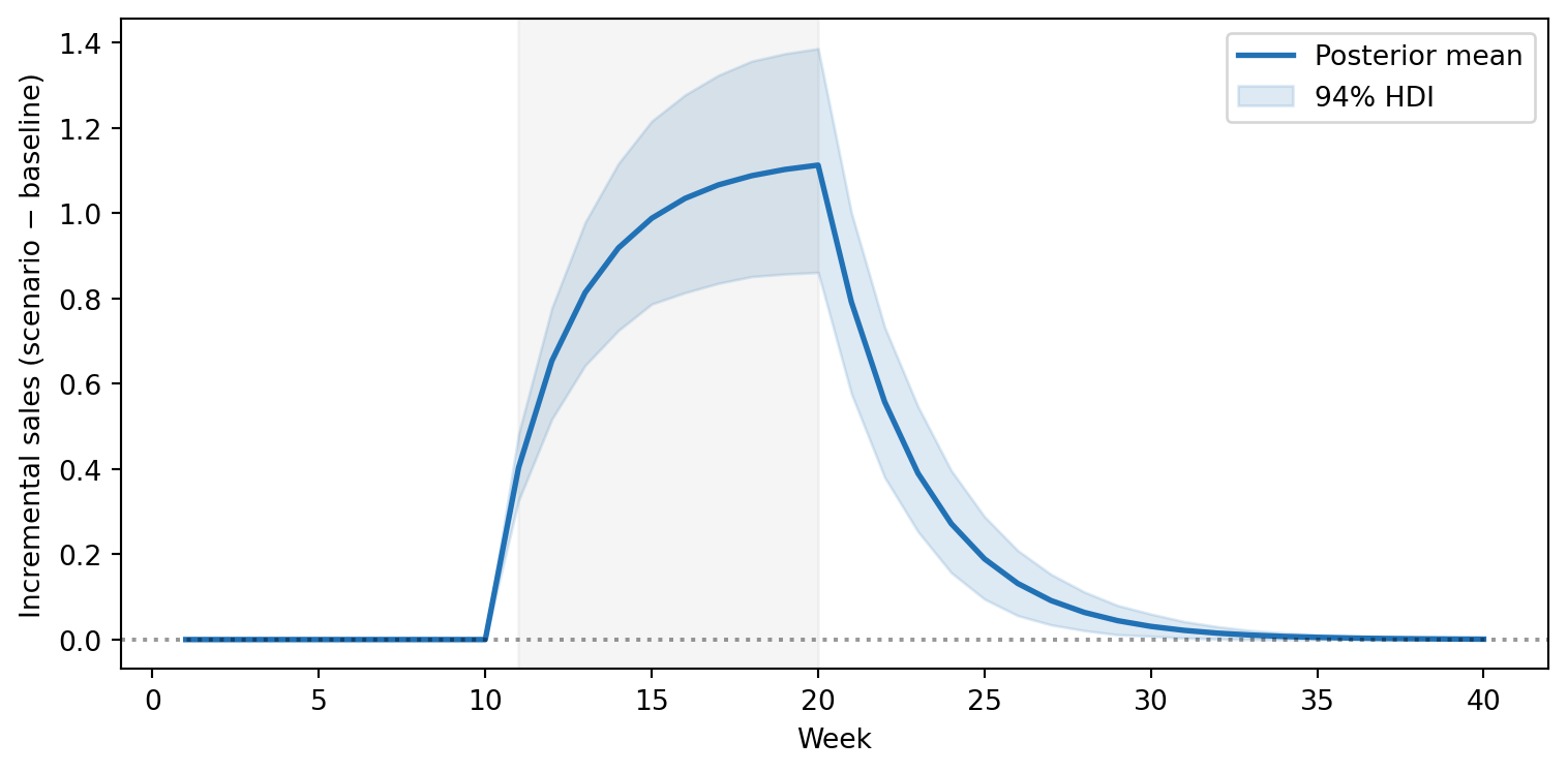

Figure 10: Incremental sales from a temporary 15% digital spend increase (weeks 11–20). Adstock causes a visible ramp-up as the stock accumulates and a gradual ramp-down as the stock decays after the boost ends.

The pattern is exactly what we expect from adstock dynamics:

Before the boost (weeks 1–10): no intervention, so the incremental effect is zero.
During the boost (weeks 11–20): the effect ramps up as the adstock stock accumulates from the extra spend.
After the boost (weeks 21+): spend returns to baseline, but the accumulated adstock decays gradually, producing a tail of residual effect.

Compare this to the AR(1) ramp-up in Figure 8: both produce gradual convergence, but through different mechanisms — adstock operates on the input (carry-over of past spend), while AR(1) operates on the outcome (persistence of the outcome itself). In practice, real systems often exhibit both.

Summary

The DAG encodes temporal assumptions. Cross-sectional DAGs have only contemporaneous edges; panel DAGs add lagged edges that represent carry-over and delayed effects.
Lagged edges create new causal paths. The total effect of a treatment can be larger than the contemporaneous effect alone, because carry-over contributes additional impact (Figure 4).
lag() syntax in the formula DSL creates lagged terms — lag(X) for lagged inputs, lag(Y) for autoregressive persistence — respecting panel boundaries automatically.
The long-run multiplier \beta_X / (1 - \rho) captures the cumulative effect of an AR(1) process, often much larger than the immediate coefficient \beta_X alone (Figure 7).
do(simulate_over="time") propagates interventions through temporal dynamics, correctly modelling ramp-up and decay for both lag terms and adstock transforms.
Partial pooling in panel models borrows strength across units, improving estimates for units with less data.
Temporal ordering aids identification. The direction of a lagged edge is unambiguous — the past cannot be caused by the future.

Reflection

Think about the causal questions in your own domain:

Marketing: does your advertising effect play out over one week or several? If you’re evaluating campaigns with a cross-sectional snapshot, could you be underestimating ROI by missing carry-over?
HR / People analytics: when a team completes a training program, does performance improve immediately, or does skill development unfold over months? A single performance review might miss the delayed effect.
Product: when you launch a new feature, does engagement spike immediately, or does adoption build as users discover it through word-of-mouth? An AR(1) model could distinguish the immediate bump from sustained momentum.

If the answer is “the effect takes time,” your DAG needs temporal edges — and that means panel data and the tools that come with it.