SaaS Conversion Funnel
Model a multi-stage conversion funnel as a causal chain to find which stage has the highest leverage on paid conversion.
Every SaaS company tracks a funnel: visitors sign up, some engage deeply, a fraction activate the product’s core features, and a smaller fraction convert to paid. The standard analytics dashboard shows conversion rates at each stage — but it cannot answer the question that matters for investment decisions: which stage of the funnel has the highest causal leverage on paid conversion?
The problem is that funnel stages are causally linked. Improving onboarding lifts engagement, which lifts activation, which lifts conversion. A naive regression of conversion on all funnel metrics simultaneously blocks the very causal paths you want to measure — the same attribution trap that plagues media mix models (see MMM with marketing funnel).
Path analysis lets us model the funnel as a causal chain, estimate the effect that propagates through each stage, and simulate “what if we improve onboarding?” scenarios that respect the full causal structure.
The causal structure
Consider a B2B SaaS product with five key variables:
- channel_quality: a score capturing how well the acquisition source matches the product’s ideal customer profile (exogenous, continuous)
- onboarding_score: quality of the onboarding experience — tutorial completion, setup wizard progress (exogenous, continuous, 1–10 scale)
- engagement: first-week activity level — sessions, feature usage, API calls (endogenous, Gaussian)
- activated: whether the user completed the product’s “aha moment” action (endogenous, Bernoulli)
- converted: whether the user became a paid subscriber within 30 days (endogenous, Bernoulli)
This DAG encodes several substantive claims:
| Path | Interpretation |
|---|---|
| onboarding → engagement → activated → converted | Full funnel: better onboarding propagates through every stage |
| onboarding → engagement → converted | Bypass path: engagement drives conversion even without formal activation |
| channel_quality → activated → converted | High-quality leads activate and convert directly |
| channel_quality → engagement → … | Channel quality also affects engagement, creating an indirect path |
ImportantMixed families in a single DAG
This model combines Gaussian and Bernoulli likelihoods in the same structural equation system. engagement is continuous (modeled with a Gaussian likelihood), while activated and converted are binary (modeled with Bernoulli-logit likelihoods). pathmc handles this automatically — each variable gets the appropriate likelihood based on the families argument, and do() applies the correct link function at each step.
Simulate data
We generate data from a known DGP so we can verify that pathmc recovers the true causal effects.
import numpy as np
import pandas as pd
import matplotlib.pyplot as plt
from scipy.special import expit
import arviz as az
import pymc as pm
import pathmc

FIG_WIDTH = 8
FIG_HEIGHT = 4
COLOR_ONBOARDING = "#2171b5"
COLOR_CHANNEL = "#e6550d"
COLOR_ENGAGEMENT = "#31a354"
COLOR_ACTIVATION = "#756bb1"
COLOR_CONVERSION = "#e7298a"

rng = np.random.default_rng(42)
n = 800

channel_quality = rng.normal(0, 1, size=n)
onboarding_score = rng.uniform(2, 9, size=n)

true_eng_intercept = 3.0
true_eng_channel = 0.6
true_eng_onboarding = 0.5

engagement = (
    true_eng_intercept
    + true_eng_channel * channel_quality
    + true_eng_onboarding * onboarding_score
    + rng.normal(scale=1.0, size=n)
)

true_act_intercept = -3.0
true_act_engagement = 0.4
true_act_channel = 0.5

logit_activated = (
    true_act_intercept
    + true_act_engagement * engagement
    + true_act_channel * channel_quality
)
p_activated = expit(logit_activated)
activated = rng.binomial(1, p_activated).astype(float)

true_conv_intercept = -3.5
true_conv_activated = 1.2
true_conv_engagement = 0.2

logit_converted = (
    true_conv_intercept
    + true_conv_activated * activated
    + true_conv_engagement * engagement
)
p_converted = expit(logit_converted)
converted = rng.binomial(1, p_converted).astype(float)

df = pd.DataFrame({
    "channel_quality": channel_quality,
    "onboarding_score": onboarding_score,
    "engagement": engagement,
    "activated": activated,
    "converted": converted,
})

print(f"N = {n}")
print(f"Activation rate:  {activated.mean():.1%}")
print(f"Conversion rate:  {converted.mean():.1%}")
print(f"Conv | activated: {converted[activated == 1].mean():.1%}")
print(f"Conv | not act:   {converted[activated == 0].mean():.1%}")
df.head()
N = 800
Activation rate: 34.4%
Conversion rate: 14.1%
Conv | activated: 25.1%
Conv | not act: 8.4%| channel_quality | onboarding_score | engagement | activated | converted | |
|---|---|---|---|---|---|
| 0 | 0.304717 | 6.275391 | 4.934083 | 1.0 | 1.0 |
| 1 | -1.039984 | 5.874786 | 3.903433 | 0.0 | 0.0 |
| 2 | 0.750451 | 4.773166 | 5.663016 | 0.0 | 1.0 |
| 3 | 0.940565 | 6.743345 | 6.206434 | 1.0 | 0.0 |
| 4 | -1.951035 | 7.080387 | 5.747544 | 0.0 | 0.0 |
The conversion rate among activated users is much higher than among non-activated users — but how much of that is causal (activation causes conversion) versus selection (engaged users both activate and convert)?
Visualise the funnel
Code
eng_quartiles = pd.qcut(df["engagement"], 4, labels=["Q1", "Q2", "Q3", "Q4"])
summary = (
    df
    .assign(eng_q=eng_quartiles)
    .groupby("eng_q")
    .agg(
        activation_rate=("activated", "mean"),
        conversion_rate=("converted", "mean"),
        n=("converted", "size"),
    )
    .reset_index()
)

fig, axes = plt.subplots(1, 2, figsize=(FIG_WIDTH, FIG_HEIGHT))

axes[0].bar(
    summary["eng_q"], summary["activation_rate"], color=COLOR_ACTIVATION, alpha=0.7
)
axes[0].set_xlabel("Engagement quartile")
axes[0].set_ylabel("Activation rate")
axes[0].set_ylim(0, 1)

axes[1].bar(
    summary["eng_q"], summary["conversion_rate"], color=COLOR_CONVERSION, alpha=0.7
)
axes[1].set_xlabel("Engagement quartile")
axes[1].set_ylabel("Conversion rate")
axes[1].set_ylim(0, 1)

plt.tight_layout()
plt.show()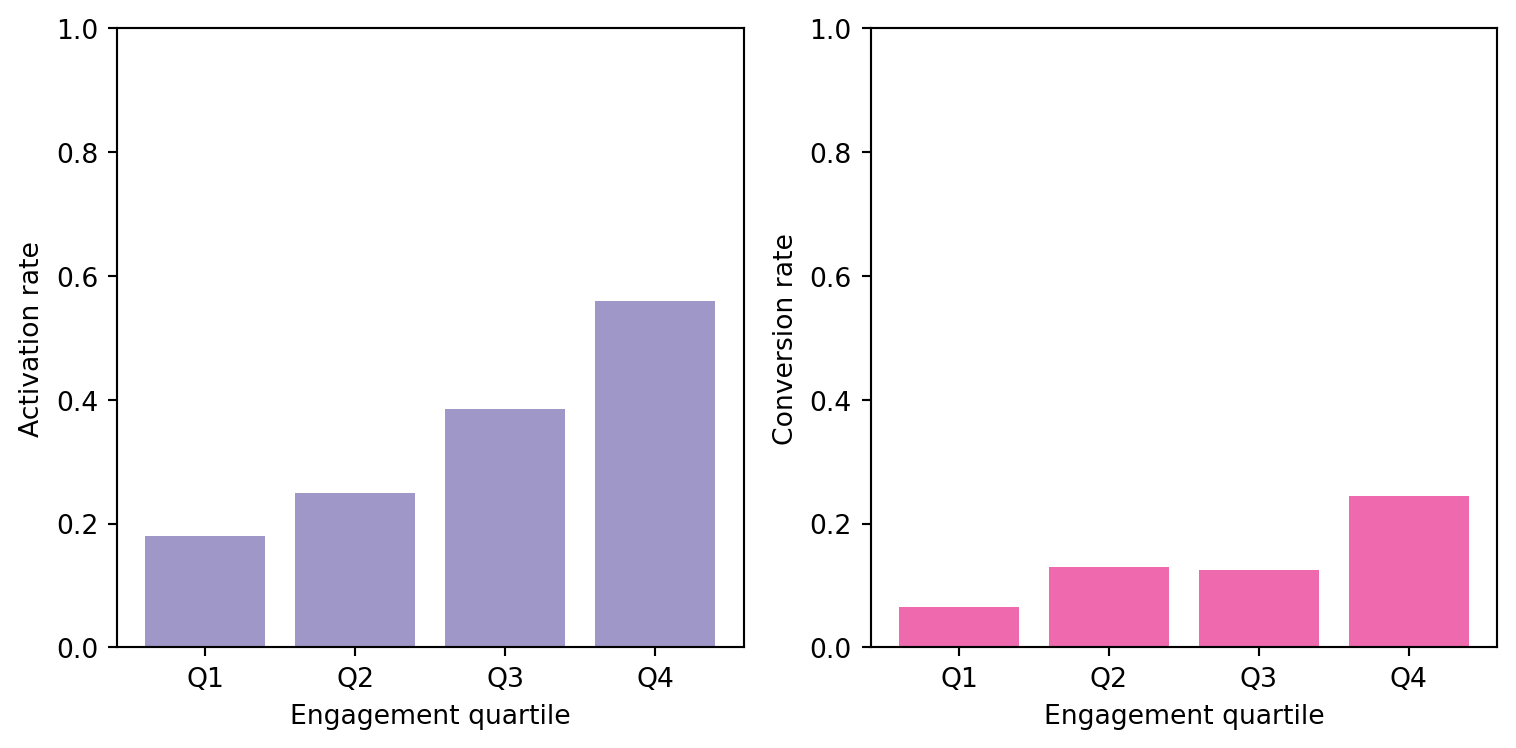
Code
fig, ax = plt.subplots(figsize=(FIG_WIDTH, FIG_HEIGHT))
mask_act = df["activated"] == 1
mask_not = df["activated"] == 0
ax.scatter(
    df.loc[mask_not, "onboarding_score"],
    df.loc[mask_not, "engagement"],
    alpha=0.3,
    s=10,
    color=COLOR_ENGAGEMENT,
    label="Not activated",
)
ax.scatter(
    df.loc[mask_act, "onboarding_score"],
    df.loc[mask_act, "engagement"],
    alpha=0.3,
    s=10,
    color=COLOR_ACTIVATION,
    label="Activated",
)
ax.set_xlabel("Onboarding score")
ax.set_ylabel("Engagement (first week)")
ax.legend()
plt.tight_layout()
plt.show()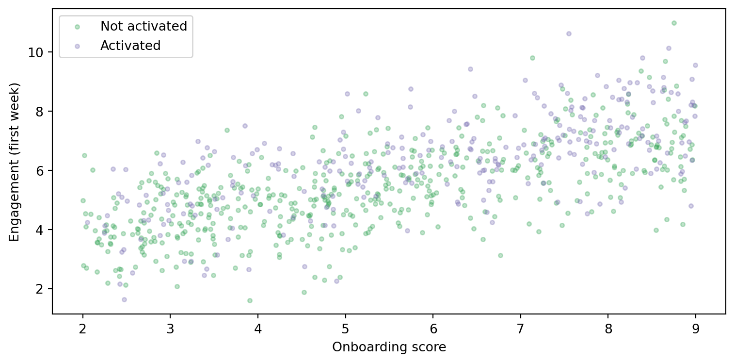
The attribution trap
Before fitting the path model, consider what a product analyst might do: regress converted on all available features simultaneously.
WarningConditioning on the mediator underestimates upstream effects
A logistic regression converted ~ onboarding_score + engagement + activated + channel_quality estimates the direct effect of onboarding on conversion — which is essentially zero, because onboarding affects conversion only through engagement and activation.
This leads to the conclusion “onboarding doesn’t matter for conversion” — a dangerous mistake if onboarding is actually the most effective lever in the entire funnel.
The same logic applies to any flat regression that includes all funnel stages as predictors: upstream variables appear irrelevant because their effects are “absorbed” by the downstream variables they cause.
Specify and fit the path model
The spec encodes the full causal chain, with each equation representing one structural relationship.
spec = """
engagement ~ e_ch*channel_quality + e_on*onboarding_score
activated  ~ a_eng*engagement + a_ch*channel_quality
converted  ~ c_act*activated + c_eng*engagement
"""

model = pathmc.model(
    spec,
    data=df,
    families={"activated": "bernoulli", "converted": "bernoulli"},
)
model.graph()
model.equations()\begin{aligned} \beta_{engagement} &\sim \text{Normal}(mu=0,\, sigma=10) \\ \sigma_{engagement} &\sim \text{HalfNormal}(sigma=1) \\ \beta_{activated} &\sim \text{Normal}(mu=0,\, sigma=10) \\ \beta_{converted} &\sim \text{Normal}(mu=0,\, sigma=10) \\[6pt] \mu_{engagement} &= \beta_{0,\,engagement} + e_{ch} \cdot \mathrm{channel\_quality} + e_{on} \cdot \mathrm{onboarding\_score} \\ \mathrm{engagement} &\sim \text{Normal}(\mu_{engagement},\, \sigma_{engagement}) \\ \mu_{activated} &= \beta_{0,\,activated} + a_{eng} \cdot \mathrm{engagement} + a_{ch} \cdot \mathrm{channel\_quality} \\ \mathrm{activated} &\sim \text{Bernoulli}(\text{logit}^{-1}(\mu_{activated})) \\ \mu_{converted} &= \beta_{0,\,converted} + c_{act} \cdot \mathrm{activated} + c_{eng} \cdot \mathrm{engagement} \\ \mathrm{converted} &\sim \text{Bernoulli}(\text{logit}^{-1}(\mu_{converted})) \end{aligned}
PyMC model graph
pm.model_to_graphviz(model.pymc_model)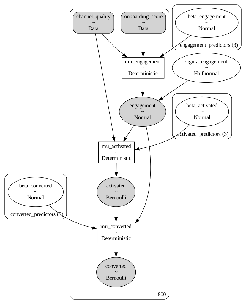
Sample
idata = model.fit(draws=1000, tune=1000, chains=4, random_seed=42)NUTS[nutpie]: [sigma_engagement, beta_engagement, beta_converted, beta_activated]Results
Coefficient recovery
model.summary()| mean | sd | eti89_lb | eti89_ub | ess_bulk | ess_tail | r_hat | mcse_mean | mcse_sd | |
|---|---|---|---|---|---|---|---|---|---|
| beta_engagement[Intercept] | 2.917461 | 0.102722 | 2.751137 | 3.082641 | 2311.481271 | 2247.234832 | 1.000975 | 0.002138 | 0.001507 |
| beta_engagement[channel_quality] | 0.604850 | 0.036388 | 0.547638 | 0.663706 | 4667.618380 | 2918.832347 | 1.002389 | 0.000535 | 0.000382 |
| beta_engagement[onboarding_score] | 0.505239 | 0.017627 | 0.476309 | 0.534019 | 2312.548542 | 2210.440597 | 1.001128 | 0.000367 | 0.000265 |
| beta_converted[Intercept] | -3.959036 | 0.444853 | -4.673583 | -3.250169 | 1829.536025 | 2250.670529 | 1.002847 | 0.010418 | 0.007184 |
| beta_converted[activated] | 1.043421 | 0.222696 | 0.687979 | 1.392330 | 4021.731178 | 2524.710551 | 1.001822 | 0.003520 | 0.002584 |
| ... | ... | ... | ... | ... | ... | ... | ... | ... | ... |
| mu_engagement[795] | 6.495892 | 0.046419 | 6.421956 | 6.569037 | 3680.939860 | 3399.277627 | 1.001567 | 0.000765 | 0.000576 |
| mu_engagement[796] | 5.844213 | 0.054061 | 5.759268 | 5.931125 | 4125.096573 | 3135.437028 | 1.000536 | 0.000842 | 0.000596 |
| mu_engagement[797] | 5.236461 | 0.066544 | 5.129140 | 5.343507 | 3301.975783 | 3158.368433 | 1.000575 | 0.001159 | 0.000806 |
| mu_engagement[798] | 5.239819 | 0.065274 | 5.134693 | 5.344699 | 3300.553682 | 3109.709021 | 1.000580 | 0.001137 | 0.000791 |
| mu_engagement[799] | 5.401681 | 0.036289 | 5.344796 | 5.460183 | 3892.693264 | 3334.777911 | 1.001676 | 0.000581 | 0.000416 |
2410 rows × 9 columns
model.effects_summary()| mean | sd | hdi_3% | hdi_97% | |
|---|---|---|---|---|
| name | ||||
| e_ch | 0.604850 | 0.036388 | 0.539363 | 0.675559 |
| e_on | 0.505239 | 0.017627 | 0.470993 | 0.537765 |
| a_eng | 0.348567 | 0.058527 | 0.239428 | 0.454937 |
| a_ch | 0.445606 | 0.094883 | 0.273171 | 0.627274 |
| c_act | 1.043421 | 0.222696 | 0.598938 | 1.436623 |
| c_eng | 0.278009 | 0.071998 | 0.148208 | 0.416253 |
TipReading the coefficients
The coefficients live on different scales depending on the family:
e_ch,e_on: identity scale (Gaussian). A one-unit increase in onboarding score increases engagement bye_on≈ 0.5 units.a_eng,a_ch: log-odds scale (Bernoulli-logit). A one-unit increase in engagement increases the log-odds of activation bya_eng≈ 0.4.c_act,c_eng: log-odds scale. Activation increases the log-odds of conversion byc_act≈ 1.2.
To get effects on the probability scale, use do() — it applies the inverse-logit transform automatically.
Identification check
print(
    f"Is onboarding → converted identifiable? {model.is_identifiable('onboarding_score', 'converted')}"
)
print(f"Adjustment sets: {model.adjustment_sets('onboarding_score', 'converted')}")
Is onboarding → converted identifiable? True
Adjustment sets: [set()]Causal effects via do()
The key business question: how much does improving onboarding increase paid conversion?
A naive regression can’t answer this because onboarding affects conversion only through engagement and activation. The do() operator propagates the intervention through the entire funnel, correctly accounting for the causal chain and the nonlinear link functions.
Total effect of onboarding on conversion
ate_onboarding = model.ate("converted", "onboarding_score", values=(3.0, 8.0))
ate_onboarding
ATE of onboarding_score on converted
| Mean | 0.10 |
| 94% HDI | [0.06, 0.14] |
| P(> 0) | 1.00 |
| Draws | 4000 |
This is the total causal effect on the probability scale — it includes the full chain: onboarding → engagement → activation → conversion, plus the bypass onboarding → engagement → conversion.
Propagation through the funnel
Because the model represents the full DAG, do() gives us the effect on every downstream variable — not just the final outcome.
r_low = model.do(set={"onboarding_score": 3.0}, kind="mean")
r_high = model.do(set={"onboarding_score": 8.0}, kind="mean")

print("do(onboarding=3) vs do(onboarding=8):")
print(
    f"  Engagement:    {r_low.mean('engagement'):.2f} → {r_high.mean('engagement'):.2f}"
)
print(
    f"  P(activated):  {r_low.mean('activated'):.3f} → {r_high.mean('activated'):.3f}"
)
print(
    f"  P(converted):  {r_low.mean('converted'):.3f} → {r_high.mean('converted'):.3f}"
)
do(onboarding=3) vs do(onboarding=8):
Engagement: 4.42 → 6.94
P(activated): 0.253 → 0.431
P(converted): 0.089 → 0.188Code
contrast = r_high - r_low

stages = ["engagement", "activated", "converted"]
stage_labels = [
    "Engagement\n(Δ units)",
    "P(Activated)\n(Δ probability)",
    "P(Converted)\n(Δ probability)",
]
colors = [COLOR_ENGAGEMENT, COLOR_ACTIVATION, COLOR_CONVERSION]

fig, axes = plt.subplots(1, 3, figsize=(FIG_WIDTH, FIG_HEIGHT))

for ax, var, label, color in zip(axes, stages, stage_labels, colors):
    draws = contrast.draws(var)
    x_kde, y_kde, _ = az.kde(draws)
    ax.plot(x_kde, y_kde, color=color, lw=2)
    ax.fill_between(x_kde, y_kde, alpha=0.3, color=color)
    ax.axvline(draws.mean(), color=color, ls="--", lw=1.5, alpha=0.7)
    ax.axvline(0, color="black", ls=":", alpha=0.3)
    ax.set_xlabel(label)
    ax.set_ylabel("Density" if ax == axes[0] else "")

plt.tight_layout()
plt.show()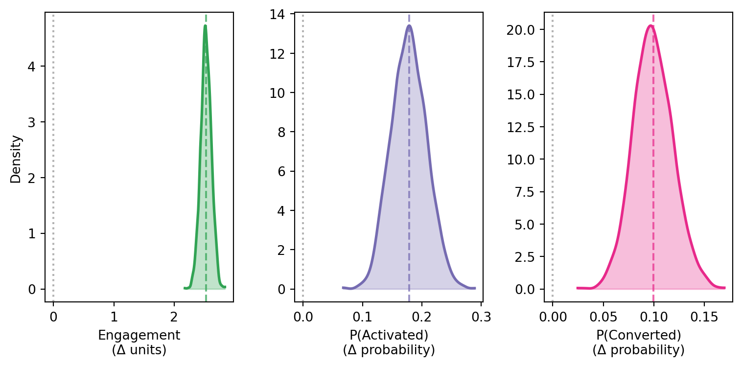
The causal cascade is visible: a 5-point improvement in onboarding lifts engagement by ~2.5 units, which increases activation probability and, in turn, conversion probability.
Which lever has the most impact?
Product teams often need to decide where to invest: improving the acquisition funnel (channel quality), the onboarding experience, or the product itself (engagement features). We can compare these by simulating comparable interventions on each lever.
r_base = model.do(set={"channel_quality": 0.0, "onboarding_score": 5.0}, kind="mean")

r_better_channel = model.do(
    set={"channel_quality": 1.0, "onboarding_score": 5.0}, kind="mean"
)
r_better_onboarding = model.do(
    set={"channel_quality": 0.0, "onboarding_score": 7.0}, kind="mean"
)

lift_channel = r_better_channel - r_base
lift_onboarding = r_better_onboarding - r_base

print("Conversion lift from 1-SD improvement in channel quality:")
print(
    f"  ΔP(converted): {lift_channel.mean('converted'):.4f}  (HDI: {lift_channel.hdi('converted', prob=0.94)})"
)
print(f"\nConversion lift from +2 onboarding score:")
print(
    f"  ΔP(converted): {lift_onboarding.mean('converted'):.4f}  (HDI: {lift_onboarding.hdi('converted', prob=0.94)})"
)
Conversion lift from 1-SD improvement in channel quality:
ΔP(converted): 0.0381 (HDI: [0.02490932 0.05156452])
Conversion lift from +2 onboarding score:
ΔP(converted): 0.0422 (HDI: [0.02488207 0.05883091])Code
fig, ax = plt.subplots(figsize=(FIG_WIDTH, FIG_HEIGHT))

for lift_obj, color, label in [
    (lift_channel, COLOR_CHANNEL, "+1 SD channel quality"),
    (lift_onboarding, COLOR_ONBOARDING, "+2 onboarding score"),
]:
    draws = lift_obj.draws("converted")
    x_kde, y_kde, _ = az.kde(draws)
    ax.plot(x_kde, y_kde, color=color, lw=2, label=label)
    ax.fill_between(x_kde, y_kde, alpha=0.25, color=color)
    ax.axvline(draws.mean(), color=color, ls="--", alpha=0.7, lw=1)

ax.axvline(0, color="black", ls=":", alpha=0.3)
ax.set_xlabel("ΔP(converted)")
ax.set_ylabel("Density")
ax.legend()
plt.tight_layout()
plt.show()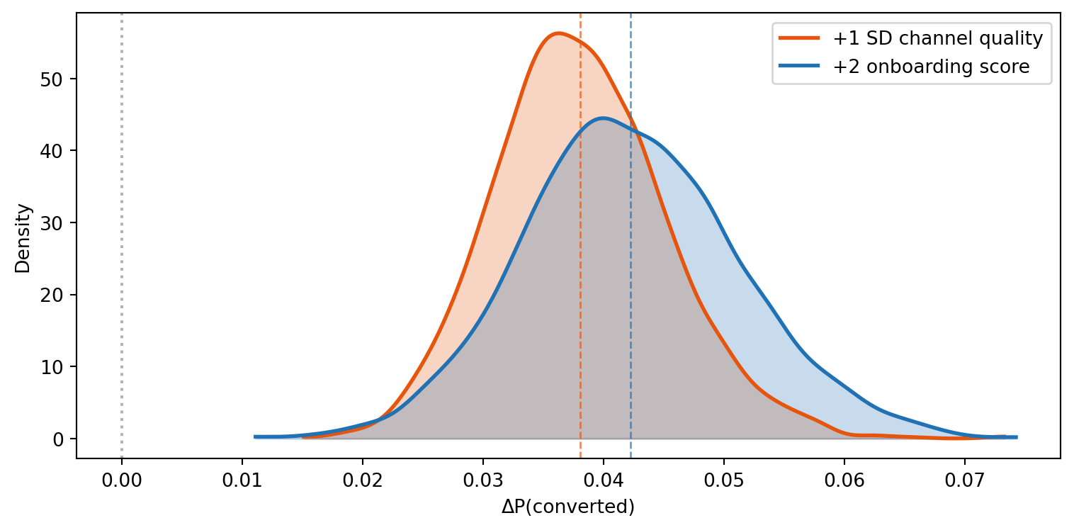
The activation question: gate or signal?
A common product debate: is activation a gate (you must activate to convert) or just a signal (engaged users both activate and convert, but activation itself doesn’t cause conversion)?
The path model can address this directly. The coefficient c_act captures the effect of activation on conversion holding engagement constant. If activation is purely a signal, this coefficient would be near zero.
Code
c_act_draws = (
    idata
    .posterior["beta_converted"]
    .sel(converted_predictors="activated")
    .values.flatten()
)

fig, ax = plt.subplots(figsize=(FIG_WIDTH, FIG_HEIGHT * 0.8))
x_kde, y_kde, _ = az.kde(c_act_draws)
ax.plot(x_kde, y_kde, color=COLOR_ACTIVATION, lw=2)
ax.fill_between(x_kde, y_kde, alpha=0.3, color=COLOR_ACTIVATION)
ax.axvline(c_act_draws.mean(), color=COLOR_ACTIVATION, ls="--", lw=1.5, alpha=0.7)
ax.axvline(
    true_conv_activated,
    color="black",
    ls="--",
    lw=1.5,
    alpha=0.5,
    label=f"True value ({true_conv_activated})",
)
ax.axvline(0, color="black", ls=":", alpha=0.3)
ax.set_xlabel("Activation → Conversion (log-odds)")
ax.set_ylabel("Density")
ax.legend()
plt.tight_layout()
plt.show()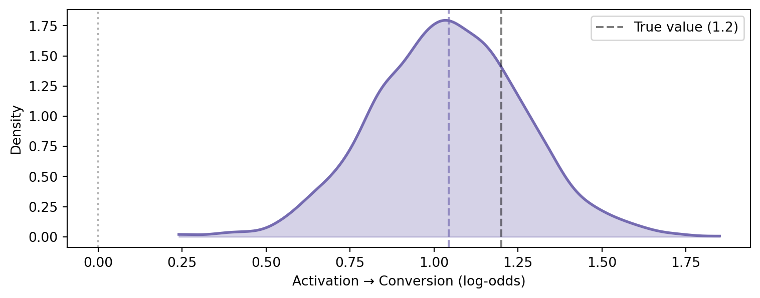
The posterior is well above zero (true value = 1.2), confirming that activation has a genuine causal effect — it’s a gate, not just a signal. This means investing in features that help users reach the “aha moment” will causally increase conversion, even holding engagement constant.
Predictive vs mean propagation
With kind="mean", the do() operator propagates expected values through the DAG. For Bernoulli variables, the “expected value” at each stage is the probability, which flows forward as a continuous number between 0 and 1.
With kind="predictive", each Bernoulli variable is sampled as an actual 0 or 1, which then flows forward as a discrete input to the next stage. This gives the full posterior predictive distribution — wider intervals, but a more faithful representation of the stochastic funnel.
r_mean = model.do(set={"onboarding_score": 8.0}, kind="mean")
r_pred = model.do(set={"onboarding_score": 8.0}, kind="predictive")

print("do(onboarding=8):")
print(
    f"  Mean propagation  — P(converted): {r_mean.mean('converted'):.3f}  "
    f"HDI: {r_mean.hdi('converted', prob=0.94)}"
)
print(
    f"  Predictive draws  — P(converted): {r_pred.mean('converted'):.3f}  "
    f"HDI: {r_pred.hdi('converted', prob=0.94)}"
)
Sampling: [activated, converted, engagement]do(onboarding=8):
Mean propagation — P(converted): 0.188 HDI: [0.15537127 0.2224477 ]
Predictive draws — P(converted): 0.193 HDI: [0. 1.]
TipWhen to use each mode
kind="mean": best for estimating causal effects and comparing scenarios. The narrower intervals isolate parameter uncertainty.kind="predictive": best for predicting what will actually happen to individual users. The wider intervals include the randomness inherent in binary outcomes.
Probability query
What fraction of users convert if we set onboarding to its maximum?
p = model.prob("converted > 0.5", set={"onboarding_score": 9.0}, kind="predictive")
print(f"P(converted | do(onboarding=9)): {p:.2f}")
/Users/benjamv/git/copilot-worktrees/pathmc/drbenvincent-literate-couscous/pathmc/_model.py:1504: UserWarning: Intervention value 9.00 for 'onboarding_score' is outside the observed data range [2.00, 9.00]. Results are extrapolations and should be interpreted with caution.
result = self.do(set=set, kind=kind, **do_kwargs)
Sampling: [activated, converted, engagement]P(converted | do(onboarding=9)): 0.22Summary
- Funnel stages are causally linked. A flat regression including all stages as predictors blocks the causal paths from upstream variables, making them appear irrelevant.
- Mixed-family models handle continuous and binary variables in the same DAG. pathmc applies the correct likelihood (Gaussian or Bernoulli-logit) to each variable automatically.
- do() propagates through the full chain. When you intervene on onboarding, the effect cascades through engagement → activation → conversion, with the logistic transform applied at each binary stage.
- Activation is a gate, not just a signal. The structural coefficient from activation to conversion is positive even after controlling for engagement, confirming a causal (not merely correlational) relationship.
- Upstream levers have larger total effects than they appear. Onboarding’s total causal effect on conversion is substantial, but invisible to a regression that conditions on the mediators.
- Mean vs predictive propagation serve different purposes: mean propagation isolates causal effects; predictive propagation gives realistic outcome distributions.
NoteReflection
In your own product or service, which metrics sit upstream in the funnel but are evaluated only by their partial correlation with the final outcome?
- Could “time to first value” be mediating the effect of onboarding investment on retention?
- Is “feature adoption” a gate to expansion revenue, or just a signal of engaged customers who would expand anyway?
- If you run an A/B test on the signup flow, does your analysis include downstream engagement metrics as covariates — accidentally blocking the very effect you’re trying to measure?