MMM with Latent Brand Awareness

Model brand awareness as a latent AR(1) mediator — first deterministic, then constrained by sparse brand-tracking surveys.

Author

Benjamin Vincent

Standard media mix models treat each channel’s effect as instantaneous (or at most, smoothed by adstock). But upper-funnel spend — brand campaigns, TV, sponsorships — doesn’t just nudge this week’s sales. It builds brand awareness, a latent stock that persists over time and compounds into sustained sales lift.

This notebook develops the idea in two parts:

Part 1 introduces the causal structure — awareness as a latent AR(1) mediator — and reveals why this model is fundamentally unidentifiable from downstream sales alone.
Part 2 shows how even sparse, noisy brand-tracking surveys solve the identification problem, enabling full posterior inference, long-run decomposition, and counterfactual analysis.

import numpy as np
import pandas as pd
import matplotlib.pyplot as plt
import arviz as az
import pathmc

FIG_WIDTH = 8
FIG_HEIGHT = 4

COLOR_UPPER = "#2171b5"
COLOR_LOWER = "#e6550d"
COLOR_AWARENESS = "#31a354"
COLOR_SURVEY = "#d62728"
COLOR_SALES = "#756bb1"
COLOR_TOTAL = "#756bb1"

Part 1: Deterministic latent awareness

Upper-funnel spend builds brand awareness — a latent stock that:

Accumulates from spend: \text{awareness}_t = a \cdot \text{upper\_funnel}_t + \rho \cdot \text{awareness}_{t-1}
Persists via an AR(1) self-loop (once built, it decays slowly)
Drives sales alongside a small direct effect from upper-funnel and a direct effect from lower-funnel

Because awareness is unobserved, the model infers its trajectory from the sales signal alone.

The causal structure

Figure 1: Brand awareness DAG. Upper-funnel spend builds awareness (a) and has a small direct effect on sales (c). Awareness persists via AR(1) dynamics (ρ) and drives sales (b). Lower-funnel spend affects sales directly (d).

Simulate data

We generate a national-level time series of 50 weeks with a known DGP so we can verify the model recovers the true parameters.

rng = np.random.default_rng(42)

n_weeks = 50

true_a = 0.5  # upper_funnel → awareness
true_rho = 0.7  # awareness persistence
true_b = 0.3  # awareness → sales
true_c = 0.2  # upper_funnel → sales (direct)
true_d = 0.5  # lower_funnel → sales
true_sigma = 1.0

rows = []
awareness = 0.0
for week in range(1, n_weeks + 1):
    uf = rng.uniform(5, 25)
    lf = rng.uniform(5, 20)
    awareness = true_a * uf + true_rho * awareness
    sales = (
        true_b * awareness + true_c * uf + true_d * lf + rng.normal(scale=true_sigma)
    )
    rows.append({
        "country": "national",
        "week": week,
        "upper_funnel": uf,
        "lower_funnel": lf,
        "sales": sales,
    })

df = pd.DataFrame(rows)

true_awareness_channel = true_a * true_b / (1 - true_rho)
true_total_uf = true_c + true_awareness_channel

df.head()

	country	week	upper_funnel	lower_funnel	sales
0	national	1	20.479121	11.583177	13.709732
1	national	2	18.947361	6.412660	10.686035
2	national	3	20.222794	16.790965	18.951347
3	national	4	14.007719	10.561970	15.531154
4	national	5	17.877302	17.341424	20.064860

If we make the simplifying assumption of a linear model with no interactions, then we can approximate the effects as below.

print(f"True upper-funnel direct effect (c):        {true_c}")
print(f"True awareness channel (a×b / (1−ρ)):       {true_awareness_channel:.3f}")
print(f"True total upper-funnel effect:              {true_total_uf:.3f}")
print(f"True lower-funnel effect (d):                {true_d}")
print(f"True awareness persistence (ρ):              {true_rho}")
print(
    f"Fraction of UF effect through awareness:     {true_awareness_channel / true_total_uf:.0%}"
)

True upper-funnel direct effect (c):        0.2
True awareness channel (a×b / (1−ρ)):       0.500
True total upper-funnel effect:              0.700
True lower-funnel effect (d):                0.5
True awareness persistence (ρ):              0.7
Fraction of UF effect through awareness:     71%

Over two-thirds of upper-funnel’s total effect on sales flows through the latent awareness stock — invisible to a model that doesn’t represent this mediator.

Visualise the data

Code

fig, axes = plt.subplots(
    2, 1, figsize=(FIG_WIDTH, FIG_HEIGHT * 1.4), sharex=True, height_ratios=[1, 1]
)

ax = axes[0]
ax.plot(df["week"], df["upper_funnel"], color=COLOR_UPPER, lw=1.2, label="Upper-funnel")
ax.plot(df["week"], df["lower_funnel"], color=COLOR_LOWER, lw=1.2, label="Lower-funnel")
ax.set_ylabel("Spend")
ax.legend(fontsize=8)
ax.set_title("Channel spend", fontweight="bold", loc="left")

ax = axes[1]
ax.plot(df["week"], df["sales"], color=COLOR_SALES, lw=1.5)
ax.scatter(df["week"], df["sales"], color=COLOR_SALES, s=15, zorder=3)
ax.set_xlabel("Week")
ax.set_ylabel("Sales")
ax.set_title("Sales", fontweight="bold", loc="left")

plt.tight_layout()
plt.show()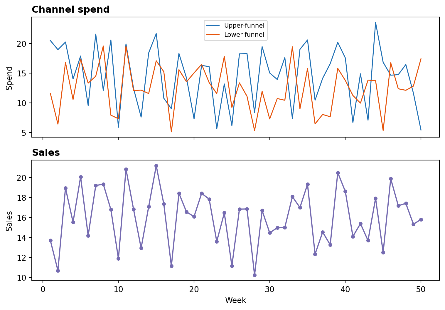

Figure 2: Simulated data over 50 weeks. Top: upper-funnel (blue) and lower-funnel (orange) weekly spend. Bottom: weekly sales, whose persistent autocorrelation reflects the latent awareness stock that accumulates from upper-funnel spend.

The attribution trap:hy naive regression undervalues upper-funnel

Regressing sales ~ upper_funnel + lower_funnel estimates the total contemporaneous association, confounding the direct effect with the awareness-mediated effect. But worse: because awareness is latent and autocorrelated, a flat regression cannot separate the persistent component from the immediate one. The model might attribute some of the awareness-driven sales to lower-funnel (if they happen to correlate), or it underestimates upper-funnel’s true ROI because the effect is spread over many future weeks.

A path model with an explicit latent awareness mediator solves both problems: it decomposes the effect and accounts for persistence.

Specify the model

The spec declares two equations: one for awareness (latent, with AR(1) persistence) and one for sales. The latent=["awareness"] argument tells pathmc that awareness is unobserved — it will be inferred as a deterministic function of the model parameters.

spec = """
awareness ~ a_uf*upper_funnel + rho*lag(awareness)
sales ~ b_aw*awareness + c_uf*upper_funnel + d_lf*lower_funnel
"""

model = pathmc.model(
    spec,
    data=df,
    panel={"unit": "country", "time": "week"},
    latent=["awareness"],
)

Why panel= and the "country" column?

The lag(awareness) term creates temporal state — each time step depends on the previous one. The panel={"unit": "country", "time": "week"} argument tells pathmc to compile a pytensor.scan loop that steps forward through time, carrying awareness as state. Even though this is a single-unit (national) model, the compiler requires both a unit and time column to set up the scan.

What latent=["awareness"] does

Because awareness is declared latent:

pathmc does not look for an awareness column in the data
The awareness equation produces a pm.Deterministic — no noise term, no likelihood
The scan propagates awareness forward through time as a carry variable: \text{awareness}_t = a \cdot \text{upper\_funnel}_t + \rho \cdot \text{awareness}_{t-1}
The only likelihood is on sales — the model infers the awareness trajectory by fitting the sales signal

model.graph()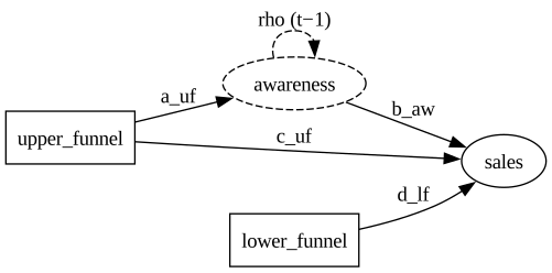

model.equations()

\begin{aligned} \beta_{awareness} &\sim \text{Normal}(mu=0,\, sigma=10) \\ \beta_{sales} &\sim \text{Normal}(mu=0,\, sigma=10) \\ \sigma_{sales} &\sim \text{HalfNormal}(sigma=1) \\[6pt] \mathrm{awareness} &\equiv \beta_{0,\,awareness} + a_{uf} \cdot \mathrm{upper\_funnel} + \rho \cdot \mathrm{lag(awareness)} \\ \mu_{sales} &= \beta_{0,\,sales} \\ &\quad + b_{aw} \cdot \mathrm{awareness} \\ &\quad + c_{uf} \cdot \mathrm{upper\_funnel} \\ &\quad + d_{lf} \cdot \mathrm{lower\_funnel} \\ \mathrm{sales} &\sim \text{Normal}(\mu_{sales},\, \sigma_{sales}) \end{aligned}

The identification problem

The model is structurally sound — the DAG is correct and the equations are well-specified. But can we actually estimate the parameters? Unrolling the awareness recursion reveals that awareness at time t is a weighted sum of all past upper-funnel spend:

\text{awareness}_t = a \sum_{k=0}^{t-1} \rho^k \cdot \text{upper\_funnel}_{t-k}

Substituting into the sales equation:

\text{sales}_t = \underbrace{(a \cdot b)}_{\text{always a product}} \sum_{k=0}^{t-1} \rho^k \cdot \text{uf}_{t-k} \;+\; c \cdot \text{uf}_t \;+\; d \cdot \text{lf}_t \;+\; \epsilon_t

The parameters a and b never appear separately in the likelihood — only their product a \cdot b matters. You can double a and halve b, or vice versa, and the model produces identical predictions. This is multiplicative non-identifiability: the data constrain the product a \cdot b and the persistence \rho, but cannot distinguish between the individual path coefficients.

Why this model cannot be sampled as-is

The non-identifiability creates a curved ridge in the (a, b) posterior: every point along the hyperbola a \cdot b = \text{const} fits the data equally well. HMC cannot efficiently explore this geometry — the sampler produces divergent transitions as it tries to traverse the narrow ridge.

Strong informative priors on a or b individually could pin the scale and break the symmetry, but this requires genuine prior knowledge about the units of the latent awareness state — knowledge we rarely have.

The quantities we care about — the awareness-mediated effect a \cdot b / (1 - \rho) and the total upper-funnel effect — depend on the product a \cdot b, which is identified. The problem is that the sampler must explore the full (a, b, \rho) space, and the ridge makes this intractable without additional information.

What if we had direct observations of the latent state? Even noisy, sparse measurements of awareness would break the symmetry: they constrain awareness on an absolute scale, which pins a (the loading from spend to awareness) and lets b (the effect of awareness on sales) be estimated separately.

Part 2: Constraining awareness with sparse surveys

Brand tracking surveys offer a way out. Even infrequent, noisy surveys that measure brand awareness every few weeks provide direct anchor points on the latent state. These anchors propagate through the AR(1) dynamics: a single observation tightens the posterior not just at that time point, but at neighboring periods too, because the autoregressive structure links them.

The result: sparse survey data can substantially reduce uncertainty on the awareness-mediated effect — the quantity that determines upper-funnel ROI.

The causal structure

Figure 3: Brand awareness DAG with sparse survey observations. Awareness is now measured by intermittent brand tracking surveys with measurement noise (σ_meas). Dashed node borders denote latent variables.

Compared to Part 1, there is one new node: awareness_survey. This is a measurement equation — a noisy, sparse observation of the latent awareness state. Weeks without a survey contribute no measurement likelihood; weeks with a survey pull the latent state toward the observed value, weighted by the measurement noise \sigma_\text{meas}.

Component	Formula	Role
State equation	\text{awareness}_t = a \cdot \text{uf}_t + \rho \cdot \text{awareness}_{t-1} + \epsilon_t	Latent dynamics with process noise
Measurement equation	\text{survey}_t = \text{awareness}_t + \eta_t	Sparse, noisy observation
Outcome equation	\text{sales}_t = b \cdot \text{awareness}_t + c \cdot \text{uf}_t + d \cdot \text{lf}_t + \nu_t	Observed sales

The process noise \epsilon_t \sim \mathcal{N}(0, \sigma_\text{state}) is what makes this a stochastic latent node — awareness is no longer a deterministic function of its parents.

Stochastic vs deterministic awareness

In Part 1, awareness is an exact function of its parents: \text{awareness}_t = a \cdot \text{uf}_t + \rho \cdot \text{awareness}_{t-1}. Here, process noise \epsilon_t makes awareness stochastic — it drifts due to unmodeled shocks (PR events, competitor actions, seasonal mood shifts). This is more realistic but harder to identify without direct observations.

Simulate data

We generate a 52-week national time series with known parameters. Awareness evolves as a stochastic AR(1) process with process noise, and brand tracking surveys observe it every 4 weeks on average.

rng = np.random.default_rng(42)

n_weeks = 52

true_a = 0.4
true_rho = 0.75
true_b = 0.3
true_c = 0.15
true_d = 0.5
true_sigma_state = 0.5
true_sigma_meas = 1.5
true_sigma_sales = 1.0

survey_weeks = sorted(rng.choice(range(4, n_weeks + 1), size=12, replace=False))

rows = []
awareness = 0.0
for week in range(1, n_weeks + 1):
    uf = rng.uniform(5, 25)
    lf = rng.uniform(5, 20)
    awareness = true_a * uf + true_rho * awareness + rng.normal(scale=true_sigma_state)
    sales = (
        true_b * awareness
        + true_c * uf
        + true_d * lf
        + rng.normal(scale=true_sigma_sales)
    )
    survey_obs = np.nan
    if week in survey_weeks:
        survey_obs = awareness + rng.normal(scale=true_sigma_meas)

    rows.append({
        "country": "national",
        "week": week,
        "upper_funnel": uf,
        "lower_funnel": lf,
        "sales": sales,
        "awareness_true": awareness,
        "awareness_survey": survey_obs,
    })

df = pd.DataFrame(rows)

true_awareness_channel = true_a * true_b / (1 - true_rho)
true_total_uf = true_c + true_awareness_channel

n_observed = df["awareness_survey"].notna().sum()
print(f"Time series: {n_weeks} weeks, {n_observed} survey observations")
print(f"Survey coverage: {n_observed / n_weeks:.0%} of weeks")
print(f"True upper-funnel direct effect (c):        {true_c}")
print(f"True awareness channel (a×b / (1−ρ)):       {true_awareness_channel:.3f}")
print(f"True total upper-funnel effect:              {true_total_uf:.3f}")
print(f"True lower-funnel effect (d):                {true_d}")
df.head(10)

Time series: 52 weeks, 12 survey observations
Survey coverage: 23% of weeks
True upper-funnel direct effect (c):        0.15
True awareness channel (a×b / (1−ρ)):       0.480
True total upper-funnel effect:              0.630
True lower-funnel effect (d):                0.5

	country	week	upper_funnel	lower_funnel	sales	awareness_true	awareness_survey
0	national	1	17.877302	17.341424	12.708418	7.384676	NaN
1	national	2	16.091696	5.957259	9.066781	12.414410	NaN
2	national	3	20.161755	10.317890	13.424713	17.986780	NaN
3	national	4	20.567670	7.919581	14.005377	21.983308	NaN
4	national	5	8.085790	15.245734	14.667107	20.792621	NaN
5	national	6	11.516507	10.556896	14.287614	20.509058	NaN
6	national	7	7.598430	12.135574	13.260822	18.008925	19.123806
7	national	8	21.653564	15.503977	17.066422	22.439696	22.787938
8	national	9	12.749568	9.324922	13.508086	22.365314	NaN
9	national	10	8.998164	5.110434	10.691573	20.517811	NaN

Visualise the data

Code

fig, axes = plt.subplots(3, 1, figsize=(FIG_WIDTH, FIG_HEIGHT * 2), sharex=True)

ax = axes[0]
ax.plot(df["week"], df["sales"], color=COLOR_SALES, lw=1.5)
ax.scatter(df["week"], df["sales"], color=COLOR_SALES, s=12, zorder=3)
ax.set_ylabel("Sales")
ax.set_title("Sales", fontweight="bold", loc="left")

ax = axes[1]
ax.plot(df["week"], df["upper_funnel"], color=COLOR_UPPER, lw=1.2, label="Upper-funnel")
ax.plot(df["week"], df["lower_funnel"], color=COLOR_LOWER, lw=1.2, label="Lower-funnel")
ax.set_ylabel("Spend")
ax.legend(fontsize=8)
ax.set_title("Channel spend", fontweight="bold", loc="left")

ax = axes[2]
ax.plot(
    df["week"],
    df["awareness_true"],
    color=COLOR_AWARENESS,
    lw=2,
    label="True awareness",
)
survey_mask = df["awareness_survey"].notna()
ax.errorbar(
    df.loc[survey_mask, "week"],
    df.loc[survey_mask, "awareness_survey"],
    yerr=true_sigma_meas,
    fmt="o",
    color=COLOR_SURVEY,
    ms=6,
    capsize=3,
    label=f"Survey (σ_meas = {true_sigma_meas})",
    zorder=4,
)
ax.set_ylabel("Awareness")
ax.set_xlabel("Week")
ax.legend(fontsize=8)
ax.set_title(
    "Latent awareness with sparse survey observations", fontweight="bold", loc="left"
)

plt.tight_layout()
plt.show()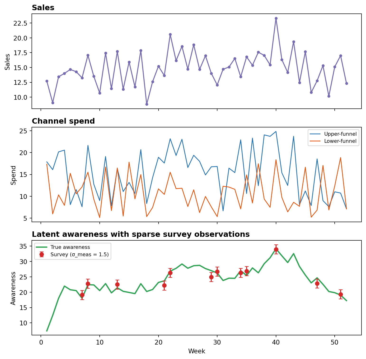

Figure 4: Simulated data with true latent awareness trajectory. Top: weekly sales. Middle: upper-funnel and lower-funnel spend. Bottom: true awareness state (green) with sparse survey observations (red points with ±1σ error bars).

Why sparse observations help

Without any survey data, the model must identify the awareness trajectory only through the sales equation — an indirect signal that also depends on lower-funnel spend, the direct upper-funnel effect, and observation noise. As Part 1 showed, this leads to multiplicative non-identifiability: the individual path coefficients a and b cannot be separated.

Survey observations change the identification picture in two ways:

Direct anchoring: At each surveyed week, the measurement likelihood pulls the latent state toward the survey value. Even noisy surveys (\sigma_\text{meas} = 1.5) reduce uncertainty relative to no observations at all.
Temporal propagation: Because awareness follows an AR(1) process, constraining the state at week t also constrains nearby weeks. A survey at week 20 narrows the posterior at weeks 18–22, not just week 20. The stronger the persistence (\rho), the further each anchor propagates.

Code

fig, ax = plt.subplots(figsize=(FIG_WIDTH, 1.5))
for w in survey_weeks:
    ax.axvline(w, color=COLOR_SURVEY, alpha=0.6, lw=2)
ax.set_xlim(0, n_weeks + 1)
ax.set_xlabel("Week")
ax.set_yticks([])
ax.set_title(
    f"{n_observed} survey observations across {n_weeks} weeks",
    fontweight="bold",
    loc="left",
)
plt.tight_layout()
plt.show()

Figure 5: Survey observation coverage across 52 weeks. Each vertical line marks a week with a brand tracking survey.

Specify and fit the model

The model has three equations: a stochastic state equation for awareness, a measurement equation linking surveys to the latent state, and the sales outcome equation.

spec = """
awareness ~ 0 + a_uf*upper_funnel + rho*lag(awareness)
sales ~ 0 + b_aw*awareness + c_uf*upper_funnel + d_lf*lower_funnel
awareness_survey ~ 0 + 1*awareness
"""

from pathmc import Prior

model = pathmc.model(
    spec,
    data=df,
    panel={"unit": "country", "time": "week"},
    latent=["awareness"],
    families={"awareness": "latent_normal"},
    priors={
        "beta_awareness": Prior("Beta", alpha=3, beta=2),
        "beta_sales": Prior("Normal", mu=0.3, sigma=0.2),
        "sigma_awareness": Prior("HalfNormal", sigma=0.5),
        "sigma_awareness_survey": Prior("HalfNormal", sigma=1.5),
        "sigma_sales": Prior("HalfNormal", sigma=1.2),
    },
)

/Users/benjamv/git/pathmc/.venv/lib/python3.12/site-packages/pymc/model/core.py:1337: ImputationWarning: Data in awareness_survey contains missing values and will be automatically imputed from the sampling distribution.
  warnings.warn(impute_message, ImputationWarning)

What the three arguments do together

latent=["awareness"] — awareness has no observed data column; the model must infer its trajectory
families={"awareness": "latent_normal"} — awareness gets process noise \sigma_\text{state} (stochastic, not deterministic)
0 + in structural equations — removes intercepts to match this simulation’s data-generating process and improve prior predictive alignment
awareness_survey ~ 0 + 1*awareness — a measurement equation with fixed loading (1) and no intercept, so survey = awareness + noise. NaN entries for unsurveyed weeks are automatically masked by PyMC

The compiler pre-generates standard-normal innovations for each time step, passes them through the scan, and scales by \sigma_\text{state}. The measurement equation is compiled as a masked likelihood — only weeks with survey data contribute to the log-probability. Here we also regularize both state noise (sigma_awareness) and measurement noise (sigma_awareness_survey) so sparse surveys more clearly anchor the latent trajectory in this teaching example. Using a bounded prior (Beta) for beta_awareness keeps both awareness coefficients in (0, 1), which helps prevent explosive AR(1)-like trajectories when fitting with sparse observations.

model.graph()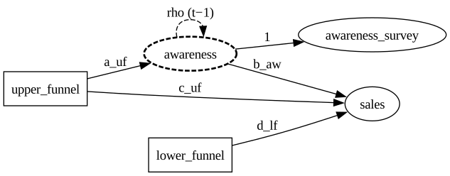

model.equations()

\begin{aligned} \beta_{awareness} &\sim \text{Beta}(alpha=3,\, beta=2) \\ \sigma_{awareness} &\sim \text{HalfNormal}(sigma=0.5) \\ \beta_{sales} &\sim \text{Normal}(mu=0.3,\, sigma=0.2) \\ \sigma_{sales} &\sim \text{HalfNormal}(sigma=1.2) \\ \sigma_{awareness,survey} &\sim \text{HalfNormal}(sigma=1.5) \\[6pt] \mu_{awareness} &= a_{uf} \cdot \mathrm{upper\_funnel} + \rho \cdot \mathrm{lag(awareness)} \\ \mathrm{awareness} &\sim \text{Normal}(\mu_{awareness},\, \sigma_{awareness}) \\ \mu_{sales} &= b_{aw} \cdot \mathrm{awareness} + c_{uf} \cdot \mathrm{upper\_funnel} + d_{lf} \cdot \mathrm{lower\_funnel} \\ \mathrm{sales} &\sim \text{Normal}(\mu_{sales},\, \sigma_{sales}) \\ \mu_{awareness,survey} &= 1 \cdot \mathrm{awareness} \\ \mathrm{awareness\_survey} &\sim \text{Normal}(\mu_{awareness,survey},\, \sigma_{awareness,survey}) \end{aligned}

model.to_graphviz()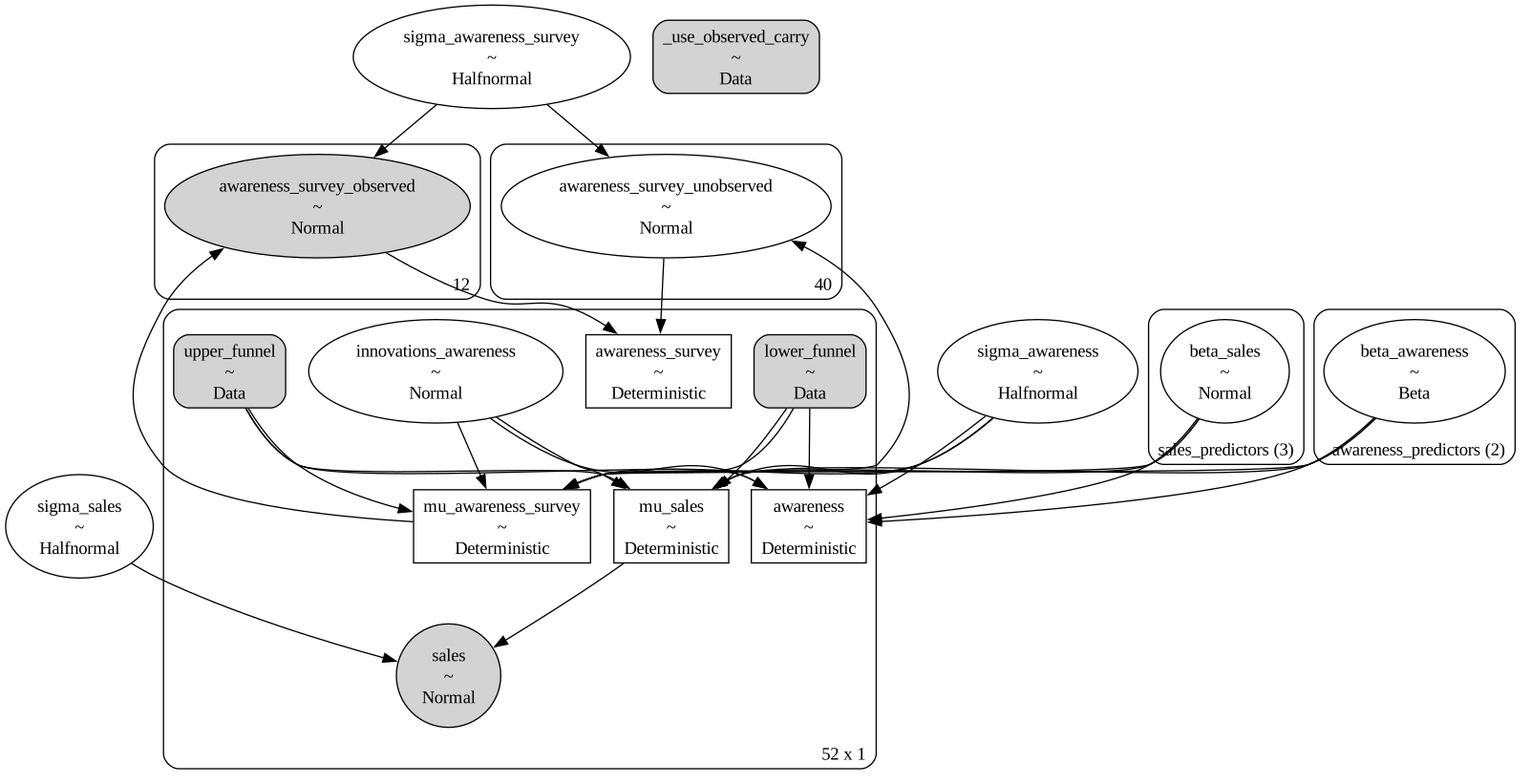

Prior predictive check

Before sampling, we draw from the prior predictive to verify that the priors generate plausible sales and awareness ranges.

Code

prior_pred = model.sample_prior_predictive(random_seed=42)
weeks = df["week"].values

fig, axes = plt.subplots(1, 2, figsize=(FIG_WIDTH, FIG_HEIGHT))

pp_mu_sales = prior_pred.prior["mu_sales"].values.reshape(-1, n_weeks)
ax = axes[0]
hdi_1 = az.hdi(pp_mu_sales, prob=0.94, axis=0)
ax.fill_between(
    weeks,
    hdi_1[:, 0],
    hdi_1[:, 1],
    alpha=0.2,
    color=COLOR_SALES,
    label="94% prior predictive",
)
ax.scatter(weeks, df["sales"], color="black", s=12, zorder=3, label="Observed")
ax.set_xlabel("Week")
ax.set_ylabel("Sales")
ax.set_title("Sales (prior predictive mean)", fontweight="bold", loc="left")
ax.legend(fontsize=8)

pp_awareness = prior_pred.prior["awareness"].values.reshape(-1, n_weeks)
ax = axes[1]
hdi_2 = az.hdi(pp_awareness, prob=0.94, axis=0)
ax.fill_between(
    weeks,
    hdi_2[:, 0],
    hdi_2[:, 1],
    alpha=0.2,
    color=COLOR_AWARENESS,
    label="94% prior predictive",
)
ax.plot(weeks, df["awareness_true"], color="black", ls="--", lw=1.5, label="True")
ax.set_xlabel("Week")
ax.set_ylabel("Awareness")
ax.set_title("Awareness", fontweight="bold", loc="left")
ax.legend(fontsize=8)

plt.tight_layout()
plt.show()

Sampling: [awareness_survey_observed, awareness_survey_unobserved, beta_awareness, beta_sales, innovations_awareness, sales, sigma_awareness, sigma_awareness_survey, sigma_sales]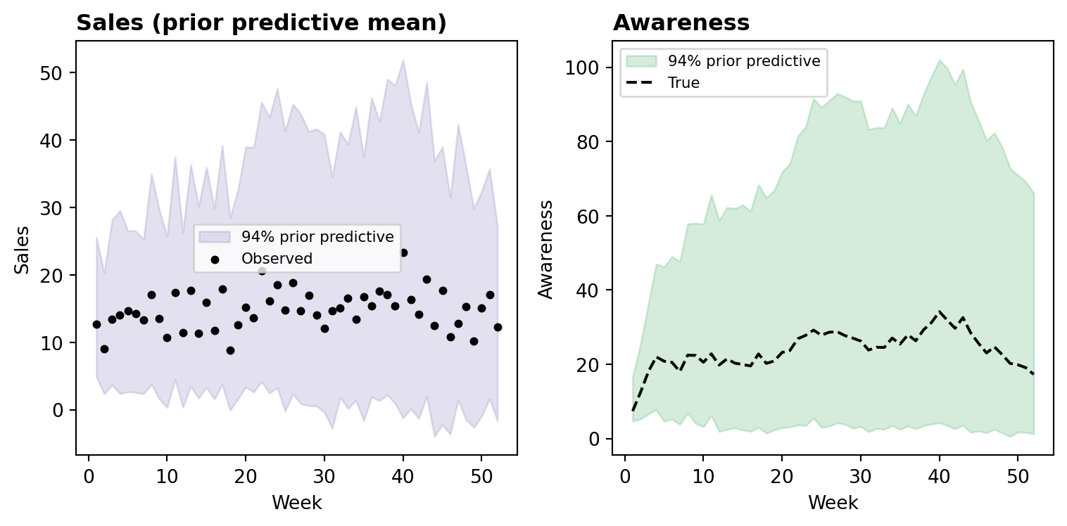

Figure 6: Prior predictive distribution of sales (left) and awareness (right). Shaded bands show the central 94% of prior-implied trajectories. The observed data (black dots) should fall within the prior predictive range — not centered, but not in the extreme tails.

Sample

idata = model.fit(
    draws=500,
    tune=1000,
    chains=4,
    cores=4,
    mp_ctx="fork",
    blas_cores=1,
    target_accept=0.99,
    nuts_sampler_kwargs={"max_treedepth": 16},
    random_seed=42,
)

/Users/benjamv/.cursor/worktrees/pathmc/pathmc-issue-263/pathmc/_model.py:658: FutureWarning: `nuts_sampler_kwargs` is deprecated. Pass NUTS keyword arguments via the `nuts={...}` argument to `pm.sample`.
  self._idata = pm.sample(**kwargs)
NUTS[nutpie]: [sigma_awareness_survey, sigma_awareness, beta_sales, beta_awareness, innovations_awareness, awareness_survey_unobserved, sigma_sales]

Sampler compatibility with sparse observations

Models with sparse measurement equations use PyMC’s masked array imputation internally — missing (NaN) positions become free random variables while observed positions contribute to the likelihood. This works seamlessly with PyMC’s built-in NUTS sampler, but nutpie (nuts_sampler="nutpie") currently fails because the masked array splitting creates unnamed shared variables that nutpie’s numba backend cannot compile. If you need nutpie’s speed for other models, note that this limitation applies specifically to models with NaN-containing observed columns. If you hit multiprocessing errors on macOS/Python 3.13 (for example RuntimeError: did not receive acknowledgement of fd), use Python 3.12 or temporarily set cores=1 as a fallback. If you see divergences, this model benefits from regularizing priors on latent dynamics and conservative NUTS settings (target_accept=0.99, higher max_treedepth), which are used in this notebook. In practice, we found a real tradeoff: aggressively tightening priors can eliminate divergences but also reduce how strongly sparse surveys recalibrate latent awareness, while looser priors improve survey tethering but can reintroduce divergences. The settings here are a pragmatic compromise for this demo.

Results

model.summary()

/Users/benjamv/git/pathmc/.venv/lib/python3.12/site-packages/arviz_stats/base/diagnostics.py:90: RuntimeWarning: invalid value encountered in scalar divide
  (between_chain_variance / within_chain_variance + num_samples - 1) / (num_samples)
/Users/benjamv/git/pathmc/.venv/lib/python3.12/site-packages/arviz_stats/base/diagnostics.py:313: RuntimeWarning: invalid value encountered in scalar divide
  varsd = varvar / evar / 4
/Users/benjamv/git/pathmc/.venv/lib/python3.12/site-packages/arviz_stats/base/diagnostics.py:313: RuntimeWarning: invalid value encountered in scalar divide
  varsd = varvar / evar / 4
/Users/benjamv/git/pathmc/.venv/lib/python3.12/site-packages/arviz_stats/base/diagnostics.py:313: RuntimeWarning: invalid value encountered in scalar divide
  varsd = varvar / evar / 4

	mean	sd	eti89_lb	eti89_ub	ess_bulk	ess_tail	r_hat	mcse_mean	mcse_sd
beta_sales[awareness]	0.323305	0.024547	0.285555	0.364512	253.660598	614.410358	1.023030	0.001551	0.001065
beta_sales[upper_funnel]	0.122062	0.034446	0.064799	0.175758	218.637979	620.351190	1.023124	0.002345	0.001710
beta_sales[lower_funnel]	0.498176	0.028914	0.452565	0.545315	2078.762140	1589.485028	1.001056	0.000631	0.000464
innovations_awareness[0, 0]	0.129015	0.957492	-1.409679	1.684244	2985.646384	1430.385466	1.001492	0.017550	0.012529
innovations_awareness[1, 0]	0.289893	0.965620	-1.276655	1.837755	2212.009218	1425.570232	1.004753	0.020684	0.014959
...	...	...	...	...	...	...	...	...	...
awareness[47, 0]	20.915620	0.982687	19.432178	22.522976	493.068156	641.843996	1.007759	0.044583	0.033737
awareness[48, 0]	19.022502	1.085494	17.401671	20.811926	266.434352	572.164538	1.017899	0.066083	0.048348
awareness[49, 0]	19.188729	1.076427	17.539229	20.984418	212.679932	404.218551	1.020440	0.072677	0.051754
awareness[50, 0]	18.970445	0.908870	17.489814	20.341715	191.699307	205.793599	1.021103	0.066312	0.046848
awareness[51, 0]	17.489212	1.236502	15.683161	19.633027	146.872568	247.538276	1.028965	0.099343	0.071838

308 rows × 9 columns

model.effects_summary()

	mean	sd	hdi_3%	hdi_97%
name
a_uf	0.406502	0.043541	0.329249	0.487122
rho	0.744697	0.029207	0.689603	0.796343
b_aw	0.323305	0.024547	0.279955	0.371293
c_uf	0.122062	0.034446	0.056716	0.185388
d_lf	0.498176	0.028914	0.444603	0.551910

Inferred awareness trajectory

Because awareness is a latent variable, the posterior contains draws of its value at every time step. Plotting the posterior mean and HDI band against the true trajectory and survey observations shows how well the model recovers the latent state — and where the surveys tighten the estimate.

Code

awareness_draws = idata.posterior["awareness"].values
awareness_flat = awareness_draws.reshape(-1, awareness_draws.shape[-2])

weeks = df["week"].values

fig, ax = plt.subplots(figsize=(FIG_WIDTH, FIG_HEIGHT))
hdi_3 = az.hdi(awareness_flat, prob=0.94, axis=0)
ax.fill_between(
    weeks, hdi_3[:, 0], hdi_3[:, 1], alpha=0.25, color=COLOR_AWARENESS, label="94% HDI"
)
ax.plot(
    weeks,
    awareness_flat.mean(axis=0),
    color=COLOR_AWARENESS,
    lw=2,
    label="Posterior mean",
)
ax.plot(
    weeks, df["awareness_true"], color="black", ls="--", lw=1.5, label="True awareness"
)

survey_mask = df["awareness_survey"].notna()
ax.errorbar(
    df.loc[survey_mask, "week"],
    df.loc[survey_mask, "awareness_survey"],
    yerr=true_sigma_meas,
    fmt="o",
    color=COLOR_SURVEY,
    ms=6,
    capsize=3,
    label=f"Survey (σ_meas = {true_sigma_meas})",
    zorder=4,
)
ax.set_xlabel("Week")
ax.set_ylabel("Awareness")
ax.legend(fontsize=8)
plt.tight_layout()
plt.show()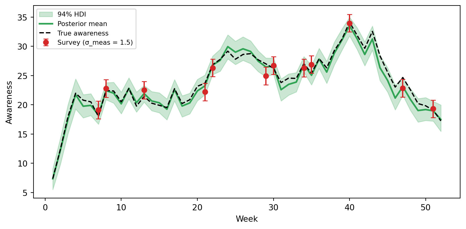

Figure 7: Inferred latent awareness trajectory (posterior mean and 94% HDI band) compared to the true awareness state (black dashed) and sparse survey observations (red points). The HDI band narrows near survey weeks.

Predicted vs observed sales

The sales equation sales ~ b*awareness + c*uf + d*lf propagates uncertainty from the latent awareness trajectory into sales predictions. Comparing the model’s posterior predictive against observed sales is a basic check that the latent structure is producing sensible downstream fit.

Code

mu_sales = idata.posterior["mu_sales"].values
mu_sales_flat = mu_sales.reshape(-1, mu_sales.shape[-2])

fig, ax = plt.subplots(figsize=(FIG_WIDTH, FIG_HEIGHT))
hdi_4 = az.hdi(mu_sales_flat, prob=0.94, axis=0)
ax.fill_between(
    weeks, hdi_4[:, 0], hdi_4[:, 1], alpha=0.25, color=COLOR_SALES, label="94% HDI"
)
ax.plot(
    weeks, mu_sales_flat.mean(axis=0), color=COLOR_SALES, lw=2, label="Posterior mean"
)
ax.scatter(weeks, df["sales"], color="black", s=15, zorder=3, label="Observed sales")
ax.set_xlabel("Week")
ax.set_ylabel("Sales")
ax.legend(fontsize=8)
plt.tight_layout()
plt.show()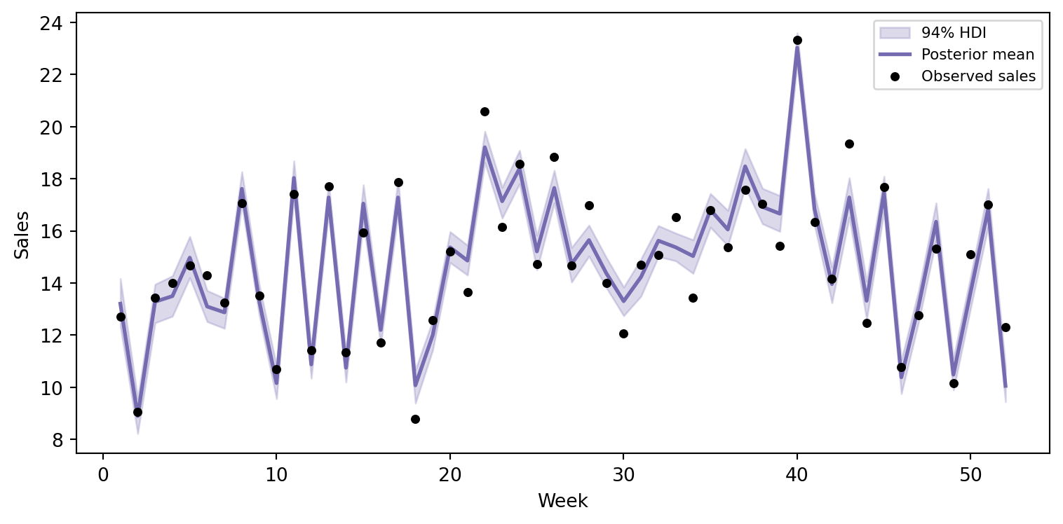

Figure 8: Posterior predictive sales (mean and 94% HDI) vs observed sales. Good coverage of the observed data indicates that the inferred awareness trajectory is consistent with the downstream sales signal.

Long-run decomposition

With the identification problem resolved by survey data, we can now decompose upper-funnel’s total long-run effect on sales into its direct path (c) and the awareness-mediated path (a \times b / (1 - \rho)). The AR(1) multiplier 1 / (1 - \rho) captures the fact that awareness persists — a single unit of spend doesn’t just affect this week’s awareness, it echoes forward through the autoregressive dynamics. Because this expression is coefficient-based, we also validate it with an intervention-based estimate in the next subsection.

Code

a_draws = (
    idata
    .posterior["beta_awareness"]
    .sel(awareness_predictors="upper_funnel")
    .values.flatten()
)
rho_draws = (
    idata
    .posterior["beta_awareness"]
    .sel(awareness_predictors="lag(awareness)")
    .values.flatten()
)
b_draws = (
    idata.posterior["beta_sales"].sel(sales_predictors="awareness").values.flatten()
)
c_draws = (
    idata.posterior["beta_sales"].sel(sales_predictors="upper_funnel").values.flatten()
)

awareness_channel_draws = a_draws * b_draws / (1 - rho_draws)
total_draws = c_draws + awareness_channel_draws

fig, ax = plt.subplots(figsize=(FIG_WIDTH, FIG_HEIGHT))

for draws, color, label, true_val in [
    (c_draws, COLOR_UPPER, "Direct (c)", true_c),
    (
        awareness_channel_draws,
        COLOR_AWARENESS,
        "Via awareness (a×b/(1−ρ))",
        true_awareness_channel,
    ),
    (total_draws, COLOR_TOTAL, "Total long-run", true_total_uf),
]:
    valid = draws[np.isfinite(draws)]
    x_kde, y_kde, _ = az.kde(valid)
    ax.plot(x_kde, y_kde, color=color, lw=2, label=label)
    ax.fill_between(x_kde, y_kde, alpha=0.25, color=color)
    ax.axvline(true_val, color=color, ls="--", lw=1.5, alpha=0.7)

ax.axvline(0, color="black", ls=":", alpha=0.3)
ax.set_xlabel("Effect on sales (per unit upper-funnel spend)")
ax.set_ylabel("Density")
ax.legend(fontsize=8)
plt.tight_layout()
plt.show()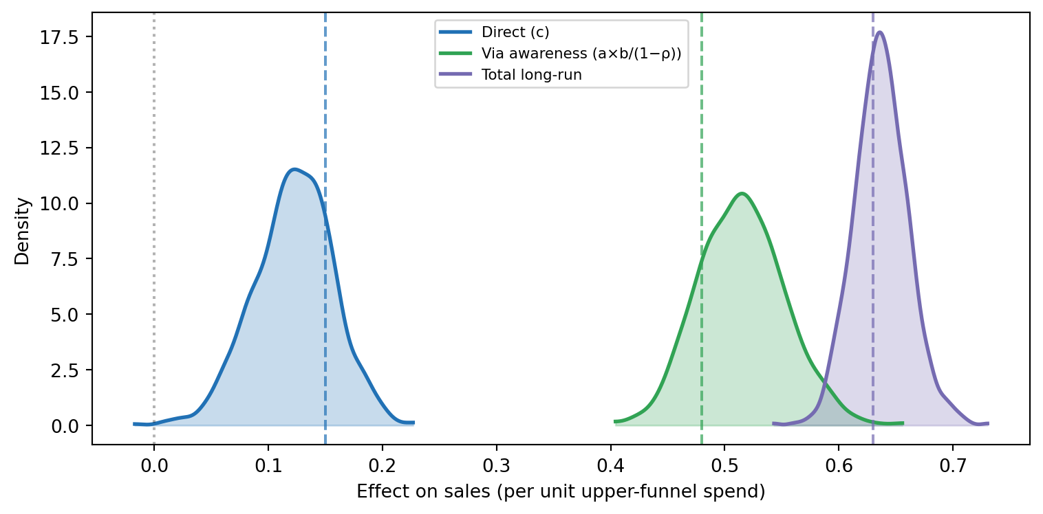

Figure 9: Posterior distributions of upper-funnel’s direct effect (c), awareness-mediated effect (a × b / (1 − ρ)), and total long-run effect. True values shown as dashed lines.

The awareness-mediated channel is larger than the direct effect — missing it means undervaluing upper-funnel by more than half. This decomposition was impossible in Part 1 because a and b were individually non-identified; here, the survey data pin awareness to an absolute scale, breaking the multiplicative degeneracy.

Validate with intervention (do())

The decomposition above uses path coefficients, which is convenient in linear AR(1) models. As a robustness check, we can estimate the same long-run quantity with intervention: set upper-funnel spend to 1 every week (vs 0), hold lower-funnel at 0 in both scenarios, and read off the stabilized sales lift from the tail of the simulated trajectory.

Code

ones_uf = np.ones(n_weeks)
zeros = np.zeros(n_weeks)

r_uf_on = model.do(
    set={"upper_funnel": ones_uf, "lower_funnel": zeros},
    simulate_over="time",
    kind="mean",
)
r_uf_off = model.do(
    set={"upper_funnel": zeros, "lower_funnel": zeros},
    simulate_over="time",
    kind="mean",
)

uf_unit_contrast = r_uf_on - r_uf_off
uf_unit_by_time = uf_unit_contrast.by_time("sales")

# Approximate steady-state lift using the final 10 weeks of the trajectory.
do_longrun_draws = uf_unit_by_time[-10:, :].mean(axis=0)

fig, ax = plt.subplots(figsize=(FIG_WIDTH, FIG_HEIGHT))
for draws, color, label in [
    (total_draws, COLOR_TOTAL, "Coefficient decomposition"),
    (do_longrun_draws, COLOR_UPPER, "Intervention (do)"),
]:
    valid = draws[np.isfinite(draws)]
    x_kde, y_kde, _ = az.kde(valid)
    ax.plot(x_kde, y_kde, color=color, lw=2, label=label)
    ax.fill_between(x_kde, y_kde, alpha=0.25, color=color)

ax.axvline(true_total_uf, color="black", ls="--", lw=1.5, alpha=0.8, label="True total")
ax.set_xlabel("Long-run sales effect per 1-unit upper-funnel spend")
ax.set_ylabel("Density")
ax.legend(fontsize=8)
plt.tight_layout()
plt.show()

/var/folders/r0/nf1kgxsx6zx3rw16xc3wnnzr0000gn/T/ipykernel_47707/2566918372.py:4: UserWarning: Intervention value [1.00, 1.00] for 'upper_funnel' is outside the observed data range [6.65, 24.85]. Results are extrapolations and should be interpreted with caution.
  r_uf_on = model.do(
/var/folders/r0/nf1kgxsx6zx3rw16xc3wnnzr0000gn/T/ipykernel_47707/2566918372.py:4: UserWarning: Intervention value [0.00, 0.00] for 'lower_funnel' is outside the observed data range [5.11, 18.87]. Results are extrapolations and should be interpreted with caution.
  r_uf_on = model.do(
/var/folders/r0/nf1kgxsx6zx3rw16xc3wnnzr0000gn/T/ipykernel_47707/2566918372.py:9: UserWarning: Intervention value [0.00, 0.00] for 'upper_funnel' is outside the observed data range [6.65, 24.85]. Results are extrapolations and should be interpreted with caution.
  r_uf_off = model.do(
/var/folders/r0/nf1kgxsx6zx3rw16xc3wnnzr0000gn/T/ipykernel_47707/2566918372.py:9: UserWarning: Intervention value [0.00, 0.00] for 'lower_funnel' is outside the observed data range [5.11, 18.87]. Results are extrapolations and should be interpreted with caution.
  r_uf_off = model.do(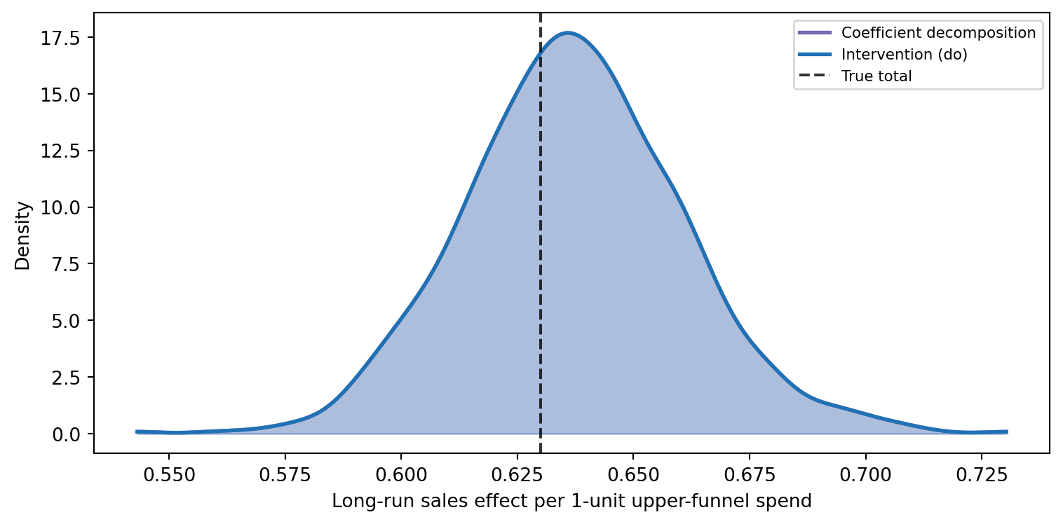

Figure 10: Long-run upper-funnel effect estimated two ways: coefficient decomposition (c + a×b/(1−ρ)) vs intervention-based g-computation from do(). In this linear model they should agree closely.

For this linear model, the two estimates should align closely. In more complex models (nonlinear transforms, interactions, non-Gaussian links), intervention-based estimation is often the safer default because it targets the causal quantity directly without relying on closed-form coefficient algebra.

Counterfactual: channel comparison over time

What does each channel contribute to sales when run at its average level versus zero?

Because awareness is persistent, upper-funnel’s contribution ramps up over time as the awareness stock builds, while lower-funnel’s contribution is flat (immediate, no persistence).

mean_uf = df["upper_funnel"].mean()
mean_lf = df["lower_funnel"].mean()

r_baseline = model.do(
    set={"upper_funnel": mean_uf},
    simulate_over="time",
    kind="mean",
)
r_no_uf = model.do(
    set={"upper_funnel": 0.0},
    simulate_over="time",
    kind="mean",
)
uf_contrast = r_baseline - r_no_uf

r_baseline_lf = model.do(
    set={"lower_funnel": mean_lf},
    simulate_over="time",
    kind="mean",
)
r_no_lf = model.do(
    set={"lower_funnel": 0.0},
    simulate_over="time",
    kind="mean",
)
lf_contrast = r_baseline_lf - r_no_lf

/var/folders/r0/nf1kgxsx6zx3rw16xc3wnnzr0000gn/T/ipykernel_47707/1525438670.py:9: UserWarning: Intervention value 0.00 for 'upper_funnel' is outside the observed data range [6.65, 24.85]. Results are extrapolations and should be interpreted with caution.
  r_no_uf = model.do(
/var/folders/r0/nf1kgxsx6zx3rw16xc3wnnzr0000gn/T/ipykernel_47707/1525438670.py:21: UserWarning: Intervention value 0.00 for 'lower_funnel' is outside the observed data range [5.11, 18.87]. Results are extrapolations and should be interpreted with caution.
  r_no_lf = model.do(

Code

fig, ax = plt.subplots(figsize=(FIG_WIDTH, FIG_HEIGHT))

weeks_seq = np.arange(1, n_weeks + 1)

uf_by_time = uf_contrast.by_time("sales")
lf_by_time = lf_contrast.by_time("sales")

ax.plot(
    weeks_seq,
    uf_by_time.mean(axis=1),
    color=COLOR_UPPER,
    lw=2,
    label="Upper-funnel contribution",
)
hdi_5 = az.hdi(uf_by_time.T, prob=0.94, axis=0)
ax.fill_between(weeks_seq, hdi_5[:, 0], hdi_5[:, 1], alpha=0.15, color=COLOR_UPPER)
ax.plot(
    weeks_seq,
    lf_by_time.mean(axis=1),
    color=COLOR_LOWER,
    lw=2,
    label="Lower-funnel contribution",
)
hdi_6 = az.hdi(lf_by_time.T, prob=0.94, axis=0)
ax.fill_between(weeks_seq, hdi_6[:, 0], hdi_6[:, 1], alpha=0.15, color=COLOR_LOWER)

ax.set_xlabel("Week")
ax.set_ylabel("Sales lift (mean spend vs. zero)")
ax.legend(fontsize=8)
ax.axhline(0, color="black", ls=":", alpha=0.3)
plt.tight_layout()
plt.show()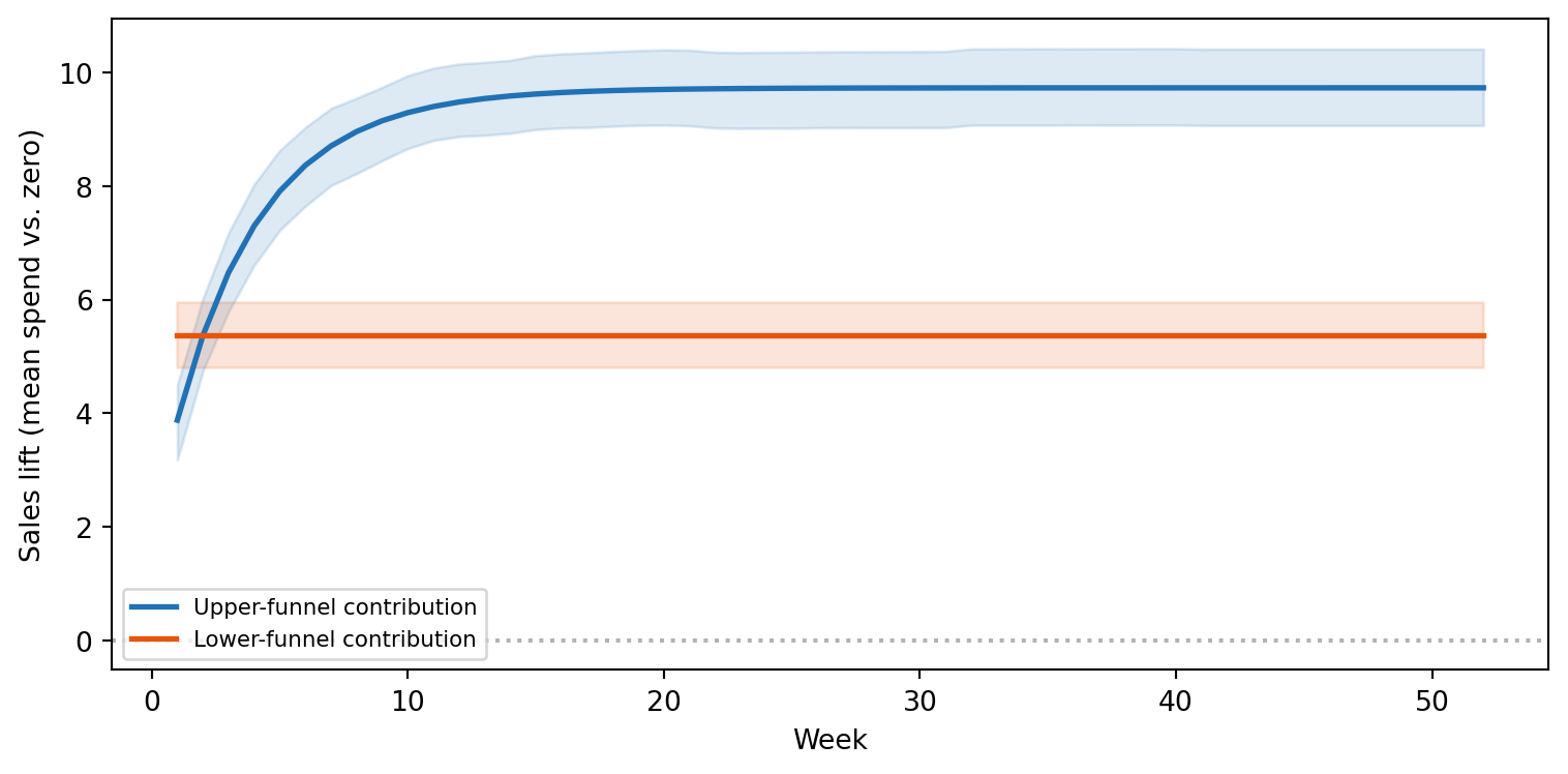

Figure 11: Impact of running each channel at its mean vs zero. Upper-funnel (blue) shows gradual ramp-up as awareness accumulates. Lower-funnel (orange) produces a flat, immediate effect with no temporal dynamics.

The asymmetry is the central insight: lower-funnel is flat (its effect is fully immediate), while upper-funnel ramps up as brand awareness builds. A snapshot at week 1 would severely underestimate upper-funnel’s contribution; by week 15+, the awareness stock has reached its long-run level.

Counterfactual: upper-funnel pulse

A brand campaign runs at high intensity for 10 weeks (weeks 11–20), then stops entirely. This produces the classic “brand halo” pattern: awareness builds during the campaign and decays slowly after it ends.

uf_pulse = np.zeros(n_weeks)
uf_pulse[10:20] = mean_uf * 2

uf_zero = np.zeros(n_weeks)

r_pulse = model.do(set={"upper_funnel": uf_pulse}, simulate_over="time", kind="mean")
r_off = model.do(set={"upper_funnel": uf_zero}, simulate_over="time", kind="mean")
pulse_effect = r_pulse - r_off

/var/folders/r0/nf1kgxsx6zx3rw16xc3wnnzr0000gn/T/ipykernel_47707/73756724.py:6: UserWarning: Intervention value [0.00, 30.55] for 'upper_funnel' is outside the observed data range [6.65, 24.85]. Results are extrapolations and should be interpreted with caution.
  r_pulse = model.do(set={"upper_funnel": uf_pulse}, simulate_over="time", kind="mean")
/var/folders/r0/nf1kgxsx6zx3rw16xc3wnnzr0000gn/T/ipykernel_47707/73756724.py:7: UserWarning: Intervention value [0.00, 0.00] for 'upper_funnel' is outside the observed data range [6.65, 24.85]. Results are extrapolations and should be interpreted with caution.
  r_off = model.do(set={"upper_funnel": uf_zero}, simulate_over="time", kind="mean")

Code

fig, ax = plt.subplots(figsize=(FIG_WIDTH, FIG_HEIGHT))

pulse_by_time = pulse_effect.by_time("sales")

ax.plot(
    weeks_seq,
    pulse_by_time.mean(axis=1),
    color=COLOR_UPPER,
    lw=2,
    label="Posterior mean",
)
hdi_7 = az.hdi(pulse_by_time.T, prob=0.94, axis=0)
ax.fill_between(
    weeks_seq, hdi_7[:, 0], hdi_7[:, 1], alpha=0.15, color=COLOR_UPPER, label="94% HDI"
)
ax.axvspan(11, 20, alpha=0.08, color="gray", label="Campaign window")
ax.axhline(0, color="black", ls=":", alpha=0.4)

ax.set_xlabel("Week")
ax.set_ylabel("Incremental sales vs. no upper-funnel")
ax.legend(fontsize=8)
plt.tight_layout()
plt.show()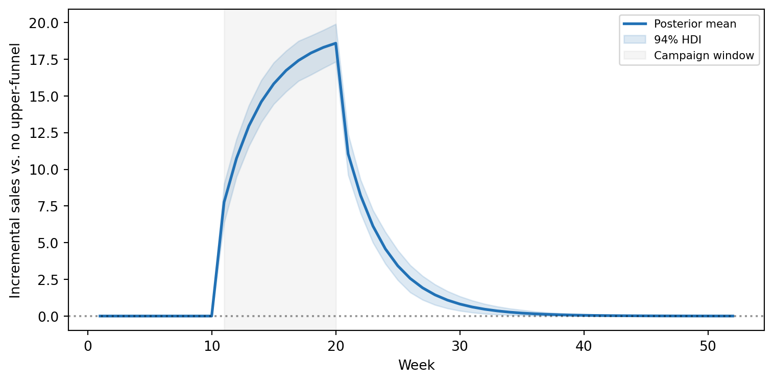

Figure 12: Sales response to a 10-week upper-funnel pulse (weeks 11–20, shaded). During the pulse, awareness accumulates and sales lift grows. After the pulse ends, the brand halo decays gradually.

This is the signature of brand awareness dynamics:

Before the campaign (weeks 1–10): no upper-funnel spend, no effect
During the campaign (weeks 11–20): awareness accumulates, sales lift ramps up
After the campaign (weeks 21+): spend stops, but the awareness stock decays at rate \rho per period — the “brand halo” sustains sales lift for many additional weeks

The total incremental sales from the pulse includes both the in-campaign lift and the post-campaign tail.

Practical considerations for survey design

The value of brand tracking surveys depends on their frequency, timing, and accuracy relative to the underlying awareness dynamics.

Frequency vs precision tradeoff: Fewer, more precise surveys (lower \sigma_\text{meas}) can be more valuable than frequent noisy ones. Each survey’s constraining power is proportional to 1 / \sigma_\text{meas}^2, while the AR(1) structure interpolates between observations.

Temporal spacing: Evenly spaced surveys provide more uniform coverage of the latent trajectory. Clustered surveys are partially redundant — the AR(1) structure means nearby observations constrain similar information.

Minimum viable coverage: Even 6–8 surveys per year (roughly monthly) can substantially improve identification, provided \rho is high enough that each observation propagates forward several weeks.

Code

fig, ax = plt.subplots(figsize=(FIG_WIDTH, FIG_HEIGHT * 0.8))

dt = np.arange(-10, 11)
for rho, ls in [(0.5, ":"), (0.75, "--"), (0.9, "-")]:
    weight = rho ** np.abs(dt)
    ax.plot(dt, weight, ls=ls, lw=2, label=f"ρ = {rho}")

ax.axvline(0, color=COLOR_SURVEY, ls="-", alpha=0.4, lw=1.5)
ax.set_xlabel("Weeks from survey observation")
ax.set_ylabel("Relative constraining effect")
ax.legend(fontsize=9)
ax.set_ylim(0, 1.05)
plt.tight_layout()
plt.show()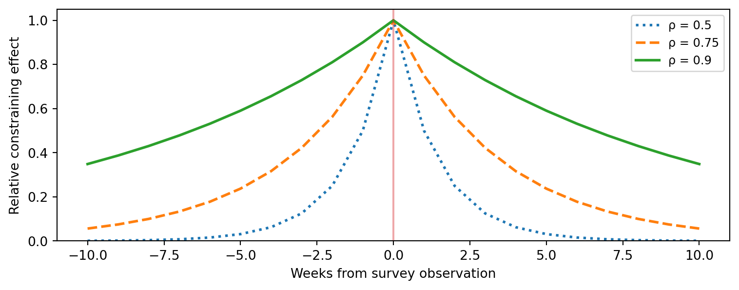

Figure 13: How a single survey observation propagates through the AR(1) structure. The constraining effect decays as ρ^|Δt| with distance from the observation, shown for three persistence values.

With \rho = 0.75 (the value in our simulation), a single survey observation retains over 30% of its constraining effect 3 weeks away and 10% at 7 weeks. Monthly surveys create overlapping zones of constraint that cover most of the year.

Summary

Brand awareness is a latent AR(1) stock. It accumulates from upper-funnel spend and decays slowly, creating persistent sales lift beyond the campaign period.
Latent mediators create multiplicative non-identifiability. When awareness is unobserved, the loading a and the effect b only appear as their product a \cdot b in the likelihood — the individual path coefficients cannot be separated from sales data alone.
Brand tracking surveys break the degeneracy. Even sparse, noisy surveys pin awareness to an absolute scale, enabling separate estimation of a and b and resolving the identification problem.
Upper-funnel effects are amplified by persistence. The direct effect c understates the total contribution; the awareness-mediated channel a \times b / (1 - \rho) captures the long-run value in this linear AR(1) setup.
Intervention-based validation is a useful complement. The long-run effect estimated from do() agrees with the coefficient decomposition here, and is often the safer default in more complex models.
Upper-funnel contribution ramps up over time; lower-funnel is flat. Because awareness accumulates, upper-funnel’s sales lift grows over weeks, while lower-funnel acts immediately with no temporal dynamics.
The “brand halo” emerges naturally from the AR(1) dynamics: a temporary campaign builds awareness that sustains sales lift for weeks after spending stops.
Even sparse surveys constrain the latent trajectory because the AR(1) structure propagates each observation’s information to neighboring time periods.
There is a practical workflow tradeoff. Tighter priors and conservative NUTS settings help reduce divergences, but overly aggressive regularization can damp survey-driven latent calibration; this notebook uses a pragmatic middle ground.

Reflection

Does your marketing data have latent stock variables that persist over time? Brand awareness is the most common example, but similar dynamics arise in:

Customer loyalty or NPS — built by service quality, persists across purchases, and mediates the effect of marketing on retention
Brand consideration in B2B — driven by thought leadership and events, decays slowly, and influences the pipeline months later
App install base — accumulated by acquisition campaigns, churns gradually, and drives in-app revenue over time

If you have sparse measurements of any of these states (quarterly surveys, periodic brand trackers), the measurement equation approach from Part 2 can substantially tighten your estimates of the channels that build them.

See the Panel Data Models example for a simpler introduction to lag() dynamics, or the Media Mix Models notebook for transforms, mediation, and hierarchical structures.