Moderation (Effect Modification)

Model treatment effect heterogeneity using interaction terms — the effect of X on Y depends on context Z.

Author

Benjamin Vincent

Does a training program improve performance equally for everyone, or does it help experienced workers more than novices? Does an ad campaign lift sales the same way in every market, or does it work better where brand awareness is already high?

These are moderation questions: the causal effect of treatment X on outcome Y depends on the level of a third variable Z — the moderator. The effect is not a single number but a function of context.

In a linear model, moderation is captured by an interaction term X \cdot Z. pathmc’s DSL supports interaction terms natively with the X:Z syntax, and the do() operator automatically recomputes the interaction product when you intervene on a constituent variable — no manual column construction needed.

The causal structure

In a moderation model, Z modifies the strength (or direction) of the X \to Y relationship. The structural equation is:

Y = \beta_0 + \beta_X X + \beta_Z Z + \beta_{XZ} X \cdot Z + \varepsilon

The conditional effect of X on Y — the causal effect at a specific level of Z — is:

\frac{\partial Y}{\partial X} = \beta_X + \beta_{XZ} \cdot Z

When \beta_{XZ} = 0, the effect of X does not depend on Z and there is no moderation. When \beta_{XZ} \neq 0, the effect is heterogeneous: it varies with the moderator.

Figure 1: Moderation DAG: both X and Z cause Y, and the X:Z interaction captures how Z modifies the strength of the X → Y effect.

Simulate data

We generate data from a known DGP so we can verify that pathmc recovers the true parameters and correctly computes conditional effects.

import numpy as np
import pandas as pd
import matplotlib.pyplot as plt
import arviz as az
import pathmc

FIG_WIDTH = 8
FIG_HEIGHT = 4
COLOR_X = "#2171b5"
COLOR_Z = "#e6550d"
COLOR_TRUE = "#333333"

rng = np.random.default_rng(42)
n = 500

TRUE_MAIN_X = 0.5
TRUE_MAIN_Z = 0.3
TRUE_INTER = 0.8

X = rng.normal(size=n)
Z = rng.normal(size=n)
Y = (
    TRUE_MAIN_X * X
    + TRUE_MAIN_Z * Z
    + TRUE_INTER * X * Z
    + rng.normal(scale=0.5, size=n)
)

df = pd.DataFrame({"X": X, "Z": Z, "Y": Y})
df.head()

	X	Z	Y
0	0.304717	1.363862	0.864350
1	-1.039984	0.895185	-1.360863
2	0.750451	-0.719480	-0.479803
3	0.940565	-1.502503	-0.794075
4	-1.951035	-2.964529	2.763740

True values: \beta_X = 0.5, \beta_Z = 0.3, \beta_{XZ} = 0.8.

The conditional effect of X at Z = z is 0.5 + 0.8z:

At Z = 0: effect = 0.5
At Z = 1: effect = 1.3
At Z = -1: effect = −0.3

So X has a strong positive effect when Z is high, and a negative effect when Z is sufficiently low (below -0.625).

Specify and fit the model

The X:Z syntax in pathmc’s DSL creates an interaction term — the element-wise product of X and Z. There is no need to precompute an interaction column in the data.

spec = """
Y ~ a*X + b*Z + c*X:Z
"""

model = pathmc.model(spec, data=df)

Inspect the model

model.graph()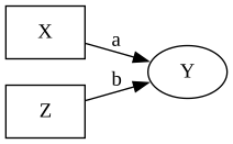

model.equations()

\begin{aligned} \beta_{Y} &\sim \text{Normal}(mu=0,\, sigma=10) \\ \sigma_{Y} &\sim \text{HalfNormal}(sigma=1) \\[6pt] \mu_{Y} &= \beta_{0,\,Y} \\ &\quad + a \cdot \mathrm{X} \\ &\quad + b \cdot \mathrm{Z} \\ &\quad + c \cdot \mathrm{X} \times \mathrm{Z} \\ \mathrm{Y} &\sim \text{Normal}(\mu_{Y},\, \sigma_{Y}) \end{aligned}

Interaction terms render as X × Z in the equation display. In the DAG, both X and Z appear as parents of Y — there is no separate node for the interaction, since it is a function of existing variables rather than an independent cause.

Sample from the posterior

idata = model.fit(draws=500, tune=500, chains=4, random_seed=42)

NUTS[nutpie]: [beta_Y, sigma_Y]

Coefficient interpretation

model.effects_summary()

	mean	sd	hdi_3%	hdi_97%
name
a	0.528523	0.024874	0.480477	0.571524
b	0.283196	0.023130	0.239210	0.325931
c	0.813939	0.024831	0.767410	0.859442

The three labeled coefficients have distinct interpretations in a moderation model:

Coefficient	Interpretation
a (\beta_X)	Effect of X on Y when Z = 0 (the “main effect” of X)
b (\beta_Z)	Effect of Z on Y when X = 0 (the “main effect” of Z)
c (\beta_{XZ})	How much the effect of X changes per unit increase in Z

Main effects are conditional, not marginal

In a model with interactions, the coefficient on X is not the average effect of X. It is the effect when Z = 0. If Z is not centered, this may not correspond to any meaningful subgroup. Centering Z before fitting ensures that the main effect of X corresponds to the effect at the sample mean of Z.

Conditional effects via cate()

The CATE at specific moderator levels

The cate() method computes the conditional average treatment effect — the causal effect of X on Y holding the moderator Z fixed at a specified value. Because pathmc knows that X:Z is a function of X and Z, it automatically recomputes the interaction product in both intervention scenarios.

for z_val in [-1.0, 0.0, 1.0]:
    cate = model.cate("Y", "X", values=(0.0, 1.0), condition={"Z": z_val})
    true_cate = TRUE_MAIN_X + TRUE_INTER * z_val
    print(
        f"CATE at Z={z_val:+.0f}:  {cate.mean():.3f}  "
        f"(true = {true_cate:.1f},  94% HDI: {cate.hdi(prob=0.94)})"
    )

CATE at Z=-1:  -0.285  (true = -0.3,  94% HDI: [-0.34888788 -0.21844517])
CATE at Z=+0:  0.529  (true = 0.5,  94% HDI: [0.4804773  0.57152392])
CATE at Z=+1:  1.342  (true = 1.3,  94% HDI: [1.26965343 1.40635375])

The estimated CATEs track the true values closely. At Z = 1, the treatment effect is strongly positive (1.3); at Z = -1, it is slightly negative (−0.3).

Effect heterogeneity: how the CATE varies with Z

The conditional effect \beta_X + \beta_{XZ} \cdot Z is a linear function of Z. We can trace out the full CATE curve by evaluating it at many moderator levels:

Code

z_grid = np.linspace(-2, 2, 30)
cate_draws_list = []

for z_val in z_grid:
    cate = model.cate("Y", "X", values=(0.0, 1.0), condition={"Z": z_val})
    cate_draws_list.append(cate.draws())

cate_draws_2d = np.column_stack(cate_draws_list)
true_cate = TRUE_MAIN_X + TRUE_INTER * z_grid

fig, ax = plt.subplots(figsize=(FIG_WIDTH, FIG_HEIGHT))

hdi_1 = az.hdi(cate_draws_2d, prob=0.94, axis=0)
ax.fill_between(z_grid, hdi_1[:, 0], hdi_1[:, 1], alpha=0.25, color=COLOR_X)
ax.plot(z_grid, cate_draws_2d.mean(axis=0), color=COLOR_X, lw=2, label="Estimated CATE")
ax.plot(z_grid, true_cate, "--", color=COLOR_TRUE, lw=2, label="True CATE")
ax.axhline(0, color="gray", lw=0.8, ls=":")
ax.set_xlabel("Moderator Z")
ax.set_ylabel("CATE of X on Y")
ax.legend()
plt.tight_layout()
plt.show()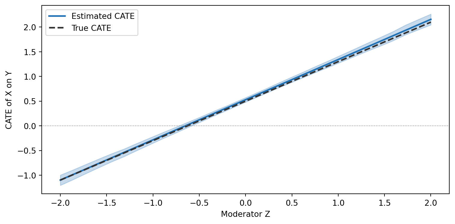

Figure 2: Conditional average treatment effect (CATE) of X on Y as a function of the moderator Z. Blue band: 94% HDI from posterior draws. Black dashed line: true conditional effect from the DGP. The treatment effect is positive for high Z and turns negative below Z ≈ −0.6.

The estimated CATE tracks the true function closely, with posterior uncertainty widening at extreme values of Z where the data is sparser.

Reading the CATE directly from coefficients

Because the model is linear, the CATE is a simple function of the posterior draws for a and c. We can verify that the cate()-based computation matches the algebraic formula:

posterior = idata.posterior.to_dataset().stack(sample=("chain", "draw"))
a_draws = posterior["beta_Y"].sel(Y_predictors="X").values
c_draws = posterior["beta_Y"].sel(Y_predictors="X:Z").values

z_check = 1.0
cate_from_coeffs = a_draws + c_draws * z_check
cate_from_cate = model.cate("Y", "X", values=(0.0, 1.0), condition={"Z": z_check})

print(f"CATE at Z=1 from coefficients: {np.mean(cate_from_coeffs):.4f}")
print(f"CATE at Z=1 from cate():       {cate_from_cate.mean():.4f}")

CATE at Z=1 from coefficients: 1.3425
CATE at Z=1 from cate():       1.3425

Both methods agree. The coefficient approach is faster (no model evaluation needed), but cate() generalizes to nonlinear models and more complex causal structures where the CATE cannot be read directly from coefficients.

Why the symbolic approach matters for do()

An alternative to the X:Z syntax is to precompute the interaction column manually:

df["XZ"] = df["X"] * df["Z"]
model_manual = pathmc.model("Y ~ a*X + b*Z + c*XZ", data=df)

This works for estimation but creates a problem for interventions: pathmc treats XZ as an independent exogenous variable with no knowledge that it derives from X and Z. When you call do(set={"X": 1.0}), the model replaces X with 1.0 but leaves XZ at its observed data values. The interaction is not recomputed, so the CATE is wrong.

With the X:Z syntax, pathmc’s compiler knows the interaction is a product of X and Z. The do() engine symbolically reconstructs X * Z from the intervened values, so interventions propagate correctly through the interaction — no manual bookkeeping required.

Rule of thumb

Use X:Z in the spec whenever the interaction involves variables you might intervene on with do(). Reserve the precomputed-column approach for interactions between strictly exogenous variables that will never be intervention targets.

ATT and ATU under moderation

When the treatment is binary and moderated by a covariate, att() and atu() provide subgroup-specific average effects that account for the different covariate distributions of the treated and untreated groups.

To demonstrate, we create a binary treatment version of the moderation model where treatment assignment depends on the moderator (confounding + effect modification):

seed = sum(map(ord, "moderation att atu"))
rng_att = np.random.default_rng(seed=seed)
n_att = 500

Z_att = rng_att.normal(size=n_att)
prob_T = 1 / (1 + np.exp(-0.8 * Z_att))
T_att = (rng_att.uniform(size=n_att) < prob_T).astype(float)

Y_att = (
    TRUE_MAIN_X * T_att
    + TRUE_MAIN_Z * Z_att
    + TRUE_INTER * T_att * Z_att
    + rng_att.normal(scale=0.5, size=n_att)
)

df_att = pd.DataFrame({"T": T_att, "Z": Z_att, "Y": Y_att})

true_att = (TRUE_MAIN_X + TRUE_INTER * Z_att[T_att == 1]).mean()
true_atu = (TRUE_MAIN_X + TRUE_INTER * Z_att[T_att == 0]).mean()

print(f"E[Z | T=1] = {Z_att[T_att == 1].mean():.2f},  True ATT = {true_att:.3f}")
print(f"E[Z | T=0] = {Z_att[T_att == 0].mean():.2f},  True ATU = {true_atu:.3f}")

E[Z | T=1] = 0.38,  True ATT = 0.801
E[Z | T=0] = -0.31,  True ATU = 0.254

Treated units have higher Z on average, and higher Z amplifies the treatment effect (positive interaction), so ATT > ATU.

model_att = pathmc.model("Y ~ a*T + b*Z + c*T:Z", data=df_att)
model_att.fit(draws=500, tune=500, chains=4, random_seed=42)

NUTS[nutpie]: [beta_Y, sigma_Y]

att = model_att.att("Y", "T")
atu = model_att.atu("Y", "T")
ate = model_att.ate("Y", "T")

print(f"{'Estimand':<12} {'Estimate':>10} {'True':>10}")
print(
    f"{'ATE':<12} {ate.mean():>10.3f} {(TRUE_MAIN_X + TRUE_INTER * Z_att.mean()):>10.3f}"
)
print(f"{'ATT':<12} {att.mean():>10.3f} {true_att:>10.3f}")
print(f"{'ATU':<12} {atu.mean():>10.3f} {true_atu:>10.3f}")

Estimand       Estimate       True
ATE               0.544      0.541
ATT               0.824      0.801
ATU               0.235      0.254

The ATT and ATU diverge because the treated group has higher Z, where the interaction amplifies the treatment effect. The cate() method fixes Z at a single value; att()/atu() average over each subgroup’s actual covariate distribution — a natural complement when treatment assignment is non-random.

Visualizing the raw data

The interaction is visible in the raw data: the slope of Y on X is steeper when Z is high than when Z is low.

Code

fig, ax = plt.subplots(figsize=(FIG_WIDTH, FIG_HEIGHT))

scatter = ax.scatter(X, Y, c=Z, cmap="viridis", alpha=0.5, s=15, rasterized=True)
plt.colorbar(scatter, ax=ax, label="Moderator Z")

ax.set_xlabel("X")
ax.set_ylabel("Y")
plt.tight_layout()
plt.show()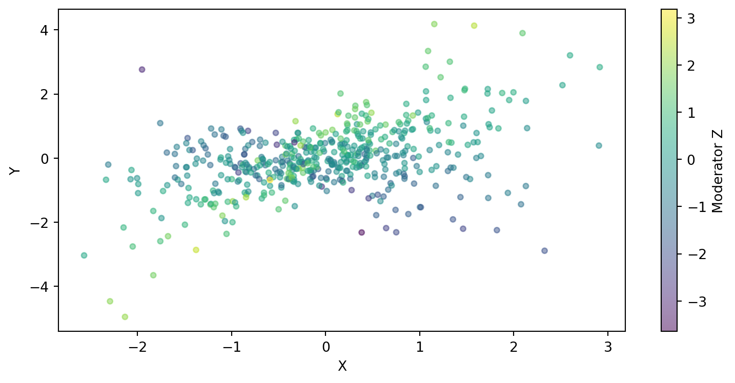

Figure 3: Y versus X, colored by the moderator Z. The slope of Y on X is steeper for high-Z observations (yellow) than for low-Z observations (purple), reflecting the positive interaction term.

Summary

Moderation (effect modification) means the causal effect of X on Y depends on a third variable Z. In a linear model, this is captured by an interaction term X \cdot Z.
pathmc’s DSL supports interactions natively with the X:Z syntax. The compiler builds the product column automatically and the do() operator recomputes it correctly under interventions.
The conditional effect of X at moderator level Z = z is \beta_X + \beta_{XZ} \cdot z. The coefficient \beta_{XZ} quantifies how much the effect changes per unit of Z.
In a model with interactions, the main effect coefficient \beta_X is the effect of X when Z = 0, not the overall average effect. Center Z if you want \beta_X to represent the effect at the sample mean.
Use model.cate("Y", "X", condition={"Z": z_val}) to compute the CATE at specific moderator levels. The do()-based CATE agrees with the algebraic formula for linear models, but generalizes to nonlinear settings.
Prefer X:Z in the spec over precomputed interaction columns when the constituent variables may be intervention targets — the symbolic approach ensures do() propagates correctly.

Reflection

Think about treatment effects in your own domain that might depend on context:

Marketing: Does advertising effectiveness depend on existing brand awareness? An ad might lift sales substantially in a market that already recognizes the brand, but have little impact where the brand is unknown.
Education: Does a new teaching method help all students equally, or does it benefit high-performers more than struggling students? The answer determines whether the method reduces or widens achievement gaps.
Medicine: Does a drug’s efficacy depend on patient age or baseline severity? If so, the average treatment effect could mask that the drug helps one subgroup substantially while doing little for another.

In each case, including the moderator as a main effect is not enough — you need the interaction term to detect how the effect varies.