import numpy as np
import pandas as pd
import matplotlib.pyplot as plt
import pathmc

FIG_WIDTH = 8
FIG_HEIGHT = 5

rng = np.random.default_rng(42)
n = 500Sensitivity to Unmeasured Confounding
How robust is your causal estimate? Quantify how strong an unmeasured confounder would need to be to overturn your conclusion.
You’ve fit a path model, adjusted for the confounders you know about, and estimated a causal effect. The credible interval excludes zero. But should you trust it?
Every causal analysis assumes no unmeasured confounders — a variable that influences both treatment and outcome but isn’t in your data. This assumption can’t be tested. Sensitivity analysis addresses it differently: rather than testing whether an unmeasured confounder exists, it asks how strong one would need to be to change your conclusion.
If overturning the result requires an implausibly strong confounder, the estimate is robust. If even a modest confounder would suffice, it’s fragile. This notebook walks through both scenarios.
Setup
A causal estimate worth defending
Consider a treatment X, an outcome Y, and an observed confounder Z that affects both. The true causal effect of X on Y is 0.5.
true_effect = 0.5

Z = rng.normal(size=n)
X = 0.6 * Z + rng.normal(scale=0.5, size=n)
Y = true_effect * X + 0.8 * Z + rng.normal(scale=0.5, size=n)

df = pd.DataFrame({"X": X, "Y": Y, "Z": Z})
The model adjusts for Z using labeled coefficients so we can inspect the individual effects later:
model = pathmc.model(
    """
    X ~ a*Z
    Y ~ b*X + c*Z
    """,
    data=df,
)
model.equations()
\begin{aligned} \beta_{X} &\sim \text{Normal}(mu=0,\, sigma=10) \\ \sigma_{X} &\sim \text{HalfNormal}(sigma=1) \\ \beta_{Y} &\sim \text{Normal}(mu=0,\, sigma=10) \\ \sigma_{Y} &\sim \text{HalfNormal}(sigma=1) \\[6pt] \mu_{X} &= \beta_{0,\,X} + a \cdot \mathrm{Z} \\ \mathrm{X} &\sim \text{Normal}(\mu_{X},\, \sigma_{X}) \\ \mu_{Y} &= \beta_{0,\,Y} + b \cdot \mathrm{X} + c \cdot \mathrm{Z} \\ \mathrm{Y} &\sim \text{Normal}(\mu_{Y},\, \sigma_{Y}) \end{aligned}
model.fit(draws=500, tune=500, chains=2, random_seed=42)NUTS[nutpie]: [beta_Y, sigma_X, beta_X, sigma_Y]<xarray.DataTree>
Group: /
├── Group: /posterior
│ Dimensions: (chain: 2, draw: 500, Y_predictors: 3, X_predictors: 2,
│ mu_Y_dim_0: 500, mu_X_dim_0: 500)
│ Coordinates:
│ * chain (chain) int64 16B 0 1
│ * draw (draw) int64 4kB 0 1 2 3 4 5 6 ... 493 494 495 496 497 498 499
│ * Y_predictors (Y_predictors) object 24B 'Intercept' 'X' 'Z'
│ * X_predictors (X_predictors) object 16B 'Intercept' 'Z'
│ * mu_Y_dim_0 (mu_Y_dim_0) int64 4kB 0 1 2 3 4 5 ... 494 495 496 497 498 499
│ * mu_X_dim_0 (mu_X_dim_0) int64 4kB 0 1 2 3 4 5 ... 494 495 496 497 498 499
│ Data variables:
│ beta_Y (chain, draw, Y_predictors) float64 24kB -0.02869 ... 0.8714
│ beta_X (chain, draw, X_predictors) float64 16kB 0.02253 ... 0.6064
│ sigma_X (chain, draw) float64 8kB 0.5186 0.5098 ... 0.4911 0.5048
│ sigma_Y (chain, draw) float64 8kB 0.5024 0.5165 ... 0.5182 0.4988
│ mu_Y (chain, draw, mu_Y_dim_0) float64 4MB 0.6409 ... -1.529
│ mu_X (chain, draw, mu_X_dim_0) float64 4MB 0.2048 ... -0.942
│ Attributes:
│ created_at: 2026-07-31T15:50:17.137839+00:00
│ creation_library: ArviZ
│ creation_library_version: 1.1.0
│ creation_library_language: Python
│ sample_dims: ['chain', 'draw']
│ inference_library: nutpie
│ inference_library_version: 0.16.10
│ sampling_time: 0.07888603210449219
│ tuning_steps: 500
├── Group: /sample_stats
│ Dimensions: (chain: 2, draw: 500)
│ Coordinates:
│ * chain (chain) int64 16B 0 1
│ * draw (draw) int64 4kB 0 1 2 3 4 ... 495 496 497 498 499
│ Data variables: (12/20)
│ depth (chain, draw) uint64 8kB 3 3 3 2 2 3 ... 2 3 2 3 3
│ maxdepth_reached (chain, draw) bool 1kB False False ... False False
│ step_size (chain, draw) float64 8kB 0.7354 0.7572 ... 0.8202
│ transformation_update_id (chain, draw) int64 8kB 0 0 0 0 0 0 ... 0 0 0 0 0
│ step_size_bar (chain, draw) float64 8kB 0.7676 0.7676 ... 0.7658
│ mean_tree_accept (chain, draw) float64 8kB 0.4049 0.8758 ... 0.9494
│ ... ...
│ fisher_distance (chain, draw) float64 8kB 0.2736 0.4647 ... 0.9199
│ transformation_index (chain, draw) int64 8kB 422 422 422 ... 423 423
│ diverging (chain, draw) bool 1kB False False ... False False
│ divergence_draw (chain, draw) uint64 8kB 0 0 0 0 0 0 ... 0 0 0 0 0
│ divergence_message (chain, draw) object 8kB None None ... None None
│ divergence_energy_error (chain, draw) float64 8kB nan nan nan ... nan nan
│ Attributes:
│ created_at: 2026-07-31T15:50:17.131780+00:00
│ creation_library: ArviZ
│ creation_library_version: 1.1.0
│ creation_library_language: Python
│ sample_dims: ['chain', 'draw']
│ inference_library: nutpie
│ inference_library_version: 0.16.10
│ inference_library_settings: {"sampler": "nuts", "adaptation": "diag", "s...
├── Group: /constant_data
│ Dimensions: (Z_dim_0: 500)
│ Coordinates:
│ * Z_dim_0 (Z_dim_0) int64 4kB 0 1 2 3 4 5 6 7 ... 493 494 495 496 497 498 499
│ Data variables:
│ Z (Z_dim_0) float64 4kB 0.3047 -1.04 0.7505 ... -0.3356 -1.991 -1.495
│ Attributes:
│ created_at: 2026-07-31T15:50:17.135149+00:00
│ creation_library: ArviZ
│ creation_library_version: 1.1.0
│ creation_library_language: Python
│ inference_library: pymc
│ inference_library_version: 6.0.1
│ sample_dims: []
├── Group: /observed_data
│ Dimensions: (X_dim_0: 500, Y_dim_0: 500)
│ Coordinates:
│ * X_dim_0 (X_dim_0) int64 4kB 0 1 2 3 4 5 6 7 ... 493 494 495 496 497 498 499
│ * Y_dim_0 (Y_dim_0) int64 4kB 0 1 2 3 4 5 6 7 ... 493 494 495 496 497 498 499
│ Data variables:
│ X (X_dim_0) float64 4kB 0.8648 -0.1764 0.09053 ... -1.129 -0.4852
│ Y (Y_dim_0) float64 4kB 0.6465 -1.285 0.4384 ... -1.801 -2.029
│ Attributes:
│ created_at: 2026-07-31T15:50:17.136659+00:00
│ creation_library: ArviZ
│ creation_library_version: 1.1.0
│ creation_library_language: Python
│ inference_library: pymc
│ inference_library_version: 6.0.1
│ sample_dims: []
└── Group: /log_likelihood
Dimensions: (chain: 2, draw: 500, X_dim_0: 500, Y_dim_0: 500)
Coordinates:
* chain (chain) int64 16B 0 1
* draw (draw) int64 4kB 0 1 2 3 4 5 6 7 ... 493 494 495 496 497 498 499
* X_dim_0 (X_dim_0) int64 4kB 0 1 2 3 4 5 6 7 ... 493 494 495 496 497 498 499
* Y_dim_0 (Y_dim_0) int64 4kB 0 1 2 3 4 5 6 7 ... 493 494 495 496 497 498 499
Data variables:
X (chain, draw, X_dim_0) float64 4MB -1.072 -0.5955 ... -0.6448
Y (chain, draw, Y_dim_0) float64 4MB -0.2307 -0.4036 ... -0.7267
Attributes:
created_at: 2026-07-31T15:50:17.225267+00:00
creation_library: ArviZ
creation_library_version: 1.1.0
creation_library_language: Python
inference_library: pymc
inference_library_version: 6.0.1
sample_dims: ['chain', 'draw']ate = model.ate("Y", "X")
print(f"True effect: {true_effect}")
ateTrue effect: 0.5ATE of X on Y
| Mean | 0.46 |
| 94% HDI | [0.38, 0.55] |
| P(> 0) | 1.00 |
| Draws | 1000 |
The ATE is well-recovered and the credible interval excludes zero. But this result assumes Z is the only confounder. What if there’s a variable we didn’t measure?
What an unmeasured confounder would do
Suppose an unobserved variable U affects both the treatment and the outcome:
If U has effect γ on treatment and δ on outcome, the estimated ATE absorbs confounding bias equal to γ × δ. The bias-corrected ATE is:
\text{adjusted ATE} = \text{observed ATE} - \gamma \times \delta
Sensitivity analysis sweeps over a grid of (γ, δ) values and finds the tipping point — the γ × δ product at which the adjusted ATE crosses zero and the causal conclusion reverses.
NoteAssumptions of this bias model
The formula adjusted ATE = observed ATE − γ × δ is a first-order approximation based on the omitted variable bias framework. It assumes U has unit variance and acts linearly on both treatment and outcome. This is the simplest parametric sensitivity model, following the tradition of Rosenbaum (2002) and VanderWeele & Ding (2017). More sophisticated approaches based on partial R² or the E-value can be layered on top.
Running the sensitivity analysis
pathmc’s sensitivity() method computes this over a grid of confounder strengths:
result = model.sensitivity("Y", "X")
result
Sensitivity Analysis — X → Y
| Observed ATE | 0.4640 [0.3826, 0.5512] (94% HDI) |
| Tipping point | γ × δ = 0.4640 |
| Symmetric example | γ = 0.6812, δ = 0.6812 would nullify the effect |
The tipping point is the γ × δ product that would exactly nullify the observed effect. The symmetric example (γ ≈ δ ≈ √tipping_point) shows what equal effects on treatment and outcome would look like.
Visualizing robustness
The .plot() method maps the adjusted ATE across the full (γ, δ) grid:
Code
fig, ax = plt.subplots(figsize=(FIG_WIDTH, FIG_HEIGHT))
result.plot(ax=ax)
plt.tight_layout()
plt.show()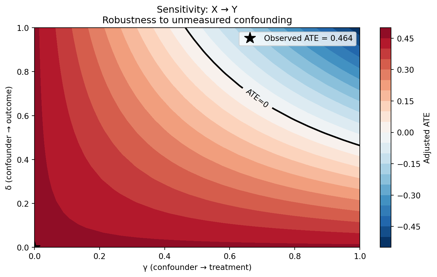
The x-axis is γ (how strongly U affects treatment), the y-axis is δ (how strongly U affects the outcome), and the color is the adjusted ATE. The black contour marks where the adjusted ATE equals zero — the tipping boundary.
Points below and to the left of the tipping line preserve a positive causal effect. Points above and to the right would reverse it. The further the tipping line sits from the origin, the more robust the effect is to unmeasured confounding.
Calibrating against observed effects
The (γ, δ) values become interpretable when compared to the effects of variables already in the model:
effects = model.effects_summary()
print(effects[["mean"]].round(3))
mean
name
a 0.596
b 0.464
c 0.849The coefficient a is the effect of Z on X; c is the direct effect of Z on Y. If an unmeasured confounder were as strong as Z, it would contribute bias of approximately a × c — comparable to the tipping point. Overturning this result would require a confounder nearly as influential as the strongest observed variable in the model.
TipCalibration heuristic
Compare the tipping point to the effects of observed variables:
- Tipping point ≫ observed effects: Robust. An unmeasured confounder would need to be far stronger than anything already measured.
- Tipping point ≈ observed effects: Borderline. A confounder comparable to known variables could explain the effect.
- Tipping point ≪ observed effects: Fragile. Even a weak unmeasured confounder could overturn the conclusion.
A fragile effect for comparison
Now consider the same confounding structure, but with a weaker true treatment effect — 0.15 instead of 0.5:
true_effect_weak = 0.15

rng2 = np.random.default_rng(123)
Z2 = rng2.normal(size=n)
X2 = 0.6 * Z2 + rng2.normal(scale=0.5, size=n)
Y2 = true_effect_weak * X2 + 0.8 * Z2 + rng2.normal(scale=0.5, size=n)

df2 = pd.DataFrame({"X": X2, "Y": Y2, "Z": Z2})

model2 = pathmc.model(
    """
    X ~ a*Z
    Y ~ b*X + c*Z
    """,
    data=df2,
)
model2.equations()
\begin{aligned} \beta_{X} &\sim \text{Normal}(mu=0,\, sigma=10) \\ \sigma_{X} &\sim \text{HalfNormal}(sigma=1) \\ \beta_{Y} &\sim \text{Normal}(mu=0,\, sigma=10) \\ \sigma_{Y} &\sim \text{HalfNormal}(sigma=1) \\[6pt] \mu_{X} &= \beta_{0,\,X} + a \cdot \mathrm{Z} \\ \mathrm{X} &\sim \text{Normal}(\mu_{X},\, \sigma_{X}) \\ \mu_{Y} &= \beta_{0,\,Y} + b \cdot \mathrm{X} + c \cdot \mathrm{Z} \\ \mathrm{Y} &\sim \text{Normal}(\mu_{Y},\, \sigma_{Y}) \end{aligned}
model2.fit(draws=500, tune=500, chains=2, random_seed=42)

ate2 = model2.ate("Y", "X")
print(f"True effect: {true_effect_weak}")
ate2
NUTS[nutpie]: [beta_Y, sigma_X, beta_X, sigma_Y]True effect: 0.15ATE of X on Y
| Mean | 0.09 |
| 94% HDI | [0.01, 0.18] |
| P(> 0) | 0.98 |
| Draws | 1000 |
The ATE is positive and the credible interval just barely excludes zero — it looks “significant.” But the sensitivity analysis reveals how fragile this conclusion is:
result2 = model2.sensitivity("Y", "X")
result2
Sensitivity Analysis — X → Y
| Observed ATE | 0.0930 [0.0086, 0.1815] (94% HDI) |
| Tipping point | γ × δ = 0.0930 |
| Symmetric example | γ = 0.3049, δ = 0.3049 would nullify the effect |
The tipping point is far smaller than in the robust case. A confounder with symmetric effects of only ~0.3 on treatment and outcome would overturn the conclusion — much weaker than the observed confounder Z.
Code
fig, ax = plt.subplots(figsize=(FIG_WIDTH, FIG_HEIGHT))
result2.plot(ax=ax)
plt.tight_layout()
plt.show()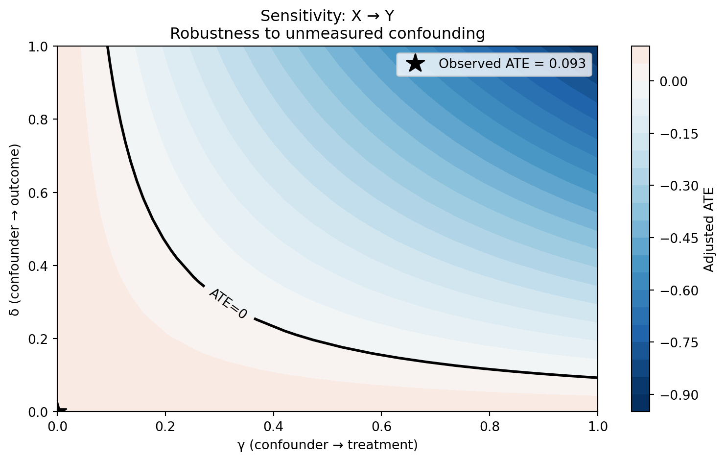
The contrast with Figure 3 is striking. The tipping line now sits much closer to the origin, meaning a wide range of plausible confounder strengths would overturn this effect. If unmeasured variables with even moderate effects on both X and Y are plausible in your domain, this causal claim should be treated with caution.
WarningWhen sensitivity analysis flags fragility
A small tipping point does not mean the effect is zero — it means the causal conclusion rests on strong identifying assumptions. The appropriate response is to:
- Seek additional data or natural experiments to rule out plausible confounders
- Report the tipping point alongside the ATE so readers can judge robustness themselves
- Identify which specific unmeasured variables could plausibly reach the tipping threshold
Summary
- Sensitivity analysis converts the untestable “no unmeasured confounders” assumption into a quantitative question: how strong would confounding need to be to change the conclusion?
- The confounding bias model assumes a latent U with effect γ on treatment and δ on outcome. The bias is γ × δ, and the adjusted ATE = observed ATE − γ × δ.
- The tipping point is the γ × δ product that reduces the ATE to zero. Larger tipping points mean more robust effects.
- The contour plot visualizes robustness across the full (γ, δ) grid. The tipping line separates the region where the causal conclusion holds from the region where it reverses.
- Calibrate the tipping point against effects of observed variables. If overturning the result requires confounders stronger than anything already measured, the effect is likely robust.
- A fragile result (small tipping point) is not necessarily wrong — it signals that the causal claim deserves additional scrutiny, ideally through complementary identification strategies.
NoteReflection
Think about a causal claim in your own work:
- What unmeasured variables could plausibly affect both the treatment and the outcome? How strong would their effects be relative to variables you already adjust for?
- In a marketing context: if you estimate the effect of a campaign on sales, could economic conditions or competitor activity act as unmeasured confounders? How large would those effects need to be to reach the tipping point?
- In a clinical setting with observational data: would a lifestyle factor like exercise or diet — correlated with both treatment adherence and health outcomes — be strong enough to overturn the estimated treatment effect?