Model-Based Data Simulation

Generate synthetic datasets from a pathmc model with known parameter values using pathmc.simulate().

Author

Benjamin Vincent

Every example in these docs simulates data with NumPy — explicit array code that anyone can audit. But pathmc can also generate data directly from a specified model, guaranteeing that the simulated dataset is perfectly consistent with the model’s generative structure.

This is useful for simulate-and-recover workflows: choose true parameter values, generate a dataset, fit the model, and verify that the posterior concentrates around truth. It is also a quick way to prototype a model before collecting real data.

The pathmc.simulate() function builds a generative PyMC model from the specification, fixes all parameters at user-provided values via pm.do(), and draws one simulated dataset.

import numpy as np
import pandas as pd
import matplotlib.pyplot as plt
import pathmc

FIG_WIDTH = 7
FIG_HEIGHT = 4

Simple regression

The simplest case: one exogenous predictor X and one outcome Y.

Figure 1: Single-equation regression: X causes Y.

Simulate

Define true parameter values and create the exogenous data. The parameter names match the PyMC model internals — beta_Y is the coefficient vector (ordered [Intercept, X]) and sigma_Y is the residual standard deviation.

seed = sum(map(ord, "simple regression"))
rng = np.random.default_rng(seed)

truth_simple = {
    "beta_Y": [2.0, 0.8],  # Intercept=2.0, slope=0.8
    "sigma_Y": 1.0,
}

n = 300
exog = pd.DataFrame({"X": rng.normal(size=n)})

df_simple = pathmc.simulate(
    "Y ~ X",
    data=exog,
    params=truth_simple,
    random_seed=rng,
)
df_simple.head()

	X	Y
0	-0.077591	2.910311
1	-0.704216	1.926878
2	-0.688257	3.130698
3	0.683797	1.672497
4	-1.683856	0.715676

The returned DataFrame contains the original exogenous column X plus the simulated outcome Y.

Code

fig, ax = plt.subplots(figsize=(FIG_WIDTH, FIG_HEIGHT))
ax.scatter(df_simple["X"], df_simple["Y"], alpha=0.3, s=15, color="C0")
x_grid = np.linspace(df_simple["X"].min(), df_simple["X"].max(), 100)
y_true = truth_simple["beta_Y"][0] + truth_simple["beta_Y"][1] * x_grid
ax.plot(x_grid, y_true, "k--", lw=2, label="True: Y = 2.0 + 0.8X")
ax.set_xlabel("X")
ax.set_ylabel("Y")
ax.legend()
plt.show()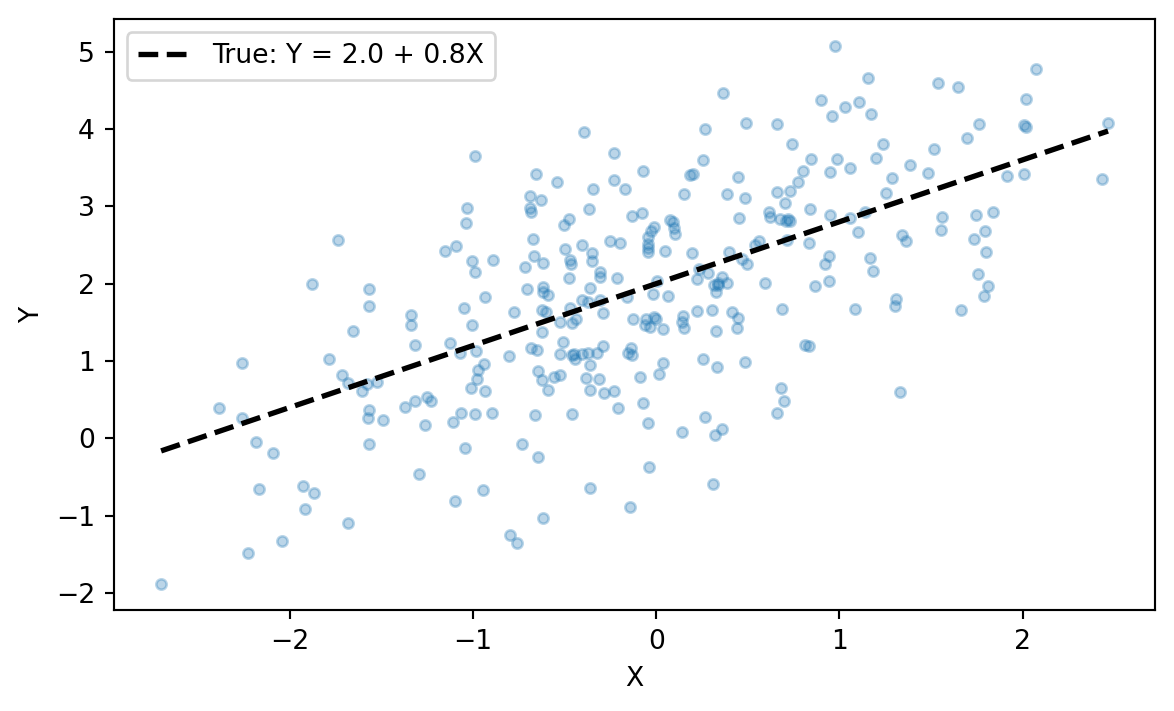

Figure 2: Simulated data from Y ~ X with known intercept (2.0) and slope (0.8). Black dashed line shows the true regression function.

Parameter recovery

Fit the model on the simulated data and check that the posterior covers the true values.

model_simple = pathmc.model("Y ~ a*X", data=df_simple)
model_simple.fit(draws=500, tune=500, chains=4, random_seed=42)
model_simple.effects_summary()

NUTS[nutpie]: [beta_Y, sigma_Y]

	mean	sd	hdi_3%	hdi_97%
name
a	0.828693	0.061863	0.725701	0.955454

The a coefficient should be close to 0.8. The full summary includes the intercept and residual scale:

model_simple.summary()

	mean	sd	eti89_lb	eti89_ub	ess_bulk	ess_tail	r_hat	mcse_mean	mcse_sd
beta_Y[Intercept]	1.925667	0.062249	1.827019	2.024299	3315.877097	1628.871077	1.002649	0.001086	0.000780
beta_Y[X]	0.828693	0.061863	0.732270	0.929139	2614.385892	1327.226896	1.003425	0.001215	0.000852
sigma_Y	1.050871	0.042616	0.984230	1.122894	3653.288475	1730.800490	1.002006	0.000705	0.000497
mu_Y[0]	1.861368	0.062120	1.762783	1.961181	3321.701060	1652.612833	1.003049	0.001083	0.000775
mu_Y[1]	1.342088	0.073603	1.224489	1.458381	3189.648140	1330.634782	1.006450	0.001301	0.000903
...	...	...	...	...	...	...	...	...	...
mu_Y[295]	-0.314207	0.174556	-0.602576	-0.036076	2814.085892	1455.186991	1.003523	0.003308	0.002208
mu_Y[296]	1.106882	0.084335	0.972580	1.238766	3130.428900	1319.471206	1.006056	0.001505	0.001026
mu_Y[297]	2.048415	0.063511	1.948679	2.152178	3272.718839	1524.931678	1.001354	0.001112	0.000806
mu_Y[298]	2.332293	0.071021	2.216512	2.448502	3140.042027	1634.580133	1.000606	0.001261	0.000939
mu_Y[299]	2.370740	0.072456	2.252185	2.489590	3106.861318	1622.455283	1.000232	0.001296	0.000968

303 rows × 9 columns

Mediation chain

A two-equation model where X affects Y both directly and indirectly through a mediator M. Simulation must generate M first, then wire it into Y’s structural equation — pathmc.simulate() handles this automatically via the generative PyMC graph.

Figure 3: Mediation DAG: X affects Y directly and indirectly through M.

Simulate

truth_med = {
    "beta_M": [0.0, 0.5],  # M = 0.0 + 0.5*X + noise
    "sigma_M": 0.5,
    "beta_Y": [1.0, 0.8, 0.3],  # Y = 1.0 + 0.8*M + 0.3*X + noise
    "sigma_Y": 0.5,
}

# Derived truths
true_indirect = truth_med["beta_M"][1] * truth_med["beta_Y"][1]  # a*b
true_direct = truth_med["beta_Y"][2]  # c
true_total = true_direct + true_indirect  # c + a*b

print(f"True indirect effect (a×b): {true_indirect:.2f}")
print(f"True direct effect (c):     {true_direct:.2f}")
print(f"True total effect:          {true_total:.2f}")

True indirect effect (a×b): 0.40
True direct effect (c):     0.30
True total effect:          0.70

exog_med = pd.DataFrame({"X": rng.normal(size=500)})

df_med = pathmc.simulate(
    """
    M ~ X
    Y ~ M + X
    """,
    data=exog_med,
    params=truth_med,
    random_seed=rng,
)
df_med.head()

	X	M	Y
0	0.674129	0.890260	1.952226
1	0.433372	-0.091577	1.564749
2	0.773107	0.273978	1.851593
3	-0.469540	-0.431065	1.050672
4	-0.317956	-0.748322	0.671664

The correlation structure should reflect the causal chain — X and M are correlated (through a), and M and Y are correlated (through b and the X → M → Y path):

df_med[["X", "M", "Y"]].corr().round(2)

	X	M	Y
X	1.00	0.72	0.73
M	0.72	1.00	0.82
Y	0.73	0.82	1.00

Parameter recovery

spec_med = """
M ~ a*X
Y ~ b*M + c*X
indirect := a*b
total := c + a*b
"""

model_med = pathmc.model(spec_med, data=df_med)
idata_med = model_med.fit(draws=500, tune=500, chains=4, random_seed=42)
model_med.effects_summary()

NUTS[nutpie]: [beta_Y, sigma_M, beta_M, sigma_Y]

	mean	sd	hdi_3%	hdi_97%
name
a	0.490741	0.021682	0.452705	0.533725
b	0.850301	0.046216	0.765042	0.939160
c	0.273248	0.032728	0.209769	0.335430
indirect	0.417290	0.029362	0.363889	0.472046
total	0.690538	0.029016	0.633719	0.743380

The indirect row should be close to {true_indirect} and total close to {true_total}. The path-specific effect API provides another way to check:

print(model_med.effect("X -> M -> Y"))
print(model_med.effect("X -> Y"))

EffectResult('X -> M -> Y', mean=0.4173, 94% HDI=[0.3639, 0.4720])
EffectResult('X -> Y', mean=0.2732, 94% HDI=[0.2098, 0.3354])

Code

import arviz as az

idata = idata_med
params_to_check = {
    "a (X→M)": ("beta_M", 1, truth_med["beta_M"][1]),
    "b (M→Y)": ("beta_Y", 1, truth_med["beta_Y"][1]),
    "c (X→Y)": ("beta_Y", 2, truth_med["beta_Y"][2]),
}

fig, axes = plt.subplots(1, 3, figsize=(FIG_WIDTH, FIG_HEIGHT * 0.8))
for ax, (label, (param, idx, true_val)) in zip(axes, params_to_check.items()):
    draws = (
        idata
        .posterior[param]
        .sel({
            f"{param.split('_')[1]}_predictors": idata
            .posterior[param]
            .coords[f"{param.split('_')[1]}_predictors"]
            .values[idx]
        })
        .values.flatten()
    )
    x_kde, y_kde, _ = az.kde(draws)
    ax.plot(x_kde, y_kde, color=None, lw=2)
    ax.fill_between(x_kde, y_kde, alpha=0.3, color=None)
    ax.axvline(true_val, color="k", ls="--", lw=1.5)
    ax.set_title(label)
    ax.set_yticks([])
fig.tight_layout()
plt.show()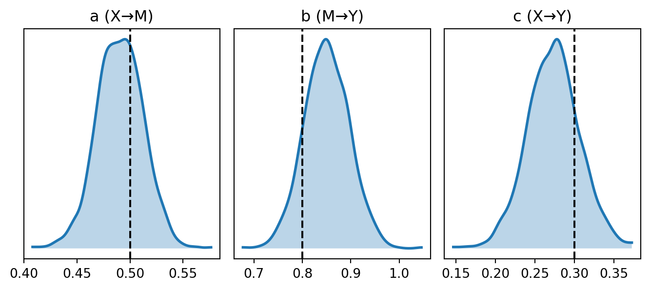

Figure 4: Parameter recovery for the mediation model. Black dashed lines mark the true values used in simulation.

Binary outcomes

Simulation works with non-Gaussian families. For a Bernoulli outcome, the coefficients are on the logit scale — the same parameterization used internally by the generative model. No separate link-function bookkeeping is needed.

Figure 5: Binary outcome model: X1 and X2 jointly predict a binary response Y.

Simulate

With Bernoulli family, there is no sigma_Y — the only parameters are the regression coefficients. The intercept controls the base log-odds, and the slopes control how each predictor shifts the probability.

truth_bin = {
    "beta_Y": [-0.5, 1.2, -0.8],  # logit(P(Y=1)) = -0.5 + 1.2*X1 - 0.8*X2
}

exog_bin = pd.DataFrame({
    "X1": rng.normal(size=500),
    "X2": rng.normal(size=500),
})

df_bin = pathmc.simulate(
    "Y ~ X1 + X2",
    data=exog_bin,
    params=truth_bin,
    families={"Y": "bernoulli"},
    random_seed=rng,
)
df_bin.head()

	X1	X2
0	-1.275853	0.316749
1	0.663898	-0.353732
2	-0.725828	0.926820
3	-0.002459	-0.722710
4	-1.101098	0.975424

print(f"Outcome prevalence: {df_bin['Y'].mean():.2%}")
print(f"Outcome values: {sorted(df_bin['Y'].unique())}")

Outcome prevalence: 43.00%
Outcome values: [np.int64(0), np.int64(1)]

Code

fig, ax = plt.subplots(figsize=(FIG_WIDTH, FIG_HEIGHT))
colors = ["C3" if y == 1 else "C0" for y in df_bin["Y"]]
ax.scatter(df_bin["X1"], df_bin["X2"], c=colors, alpha=0.3, s=15)

# Decision boundary: -0.5 + 1.2*X1 - 0.8*X2 = 0  →  X2 = (-0.5 + 1.2*X1) / 0.8
x1_grid = np.linspace(df_bin["X1"].min(), df_bin["X1"].max(), 100)
x2_boundary = (truth_bin["beta_Y"][0] + truth_bin["beta_Y"][1] * x1_grid) / -truth_bin[
    "beta_Y"
][2]
ax.plot(x1_grid, x2_boundary, "k--", lw=2, label="Decision boundary (P=0.5)")
ax.set_xlabel("X1")
ax.set_ylabel("X2")

from matplotlib.lines import Line2D

legend_elements = [
    Line2D(
        [0],
        [0],
        marker="o",
        color="w",
        markerfacecolor="C0",
        markersize=8,
        label="Y = 0",
    ),
    Line2D(
        [0],
        [0],
        marker="o",
        color="w",
        markerfacecolor="C3",
        markersize=8,
        label="Y = 1",
    ),
    Line2D([0], [0], color="k", ls="--", lw=2, label="Decision boundary"),
]
ax.legend(handles=legend_elements)
plt.show()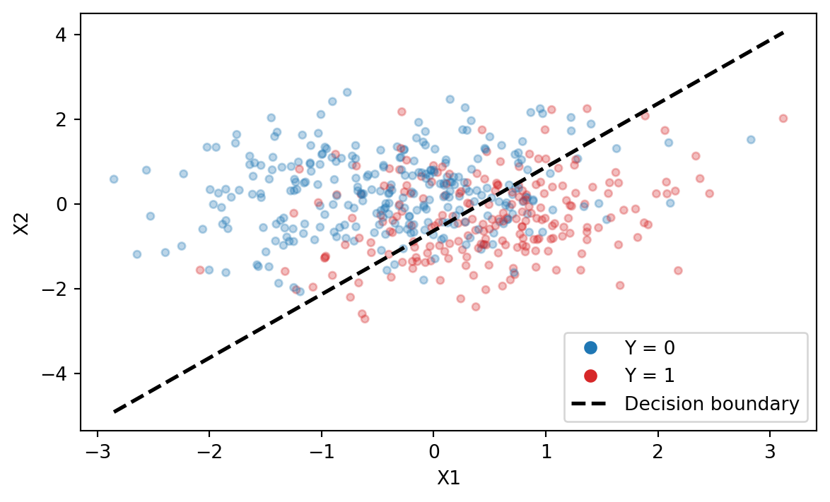

Figure 6: Simulated binary outcome colored by Y. The decision boundary (P(Y=1) = 0.5) is shown as a black dashed line.

Parameter recovery

model_bin = pathmc.model("Y ~ X1 + X2", data=df_bin, families={"Y": "bernoulli"})
model_bin.fit(draws=500, tune=500, chains=4, random_seed=42)
model_bin.summary()

NUTS[nutpie]: [beta_Y]

	mean	sd	eti89_lb	eti89_ub	ess_bulk	ess_tail	r_hat	mcse_mean	mcse_sd
beta_Y[Intercept]	-0.423581	0.110522	-0.602959	-0.249750	2201.652938	1747.445505	1.001353	0.002355	0.001662
beta_Y[X1]	1.364327	0.144049	1.129132	1.604036	1914.158392	1570.612874	1.002202	0.003298	0.002290
beta_Y[X2]	-0.980265	0.128520	-1.192692	-0.782510	2009.385378	1549.748439	1.002105	0.002877	0.001987
mu_Y[0]	-2.474758	0.249129	-2.892911	-2.080857	1574.349415	1550.562404	1.002635	0.006331	0.004352
mu_Y[1]	0.828944	0.144355	0.596793	1.065242	2751.684649	1630.230600	1.000563	0.002740	0.001976
...	...	...	...	...	...	...	...	...	...
mu_Y[495]	-3.066036	0.300722	-3.574181	-2.614002	1546.112579	1369.731784	1.006543	0.007759	0.005408
mu_Y[496]	0.799176	0.150518	0.564620	1.041981	2667.682320	1698.371719	1.001703	0.002911	0.002101
mu_Y[497]	-0.772429	0.154461	-1.020034	-0.539734	2165.165438	1606.434834	1.002345	0.003312	0.002262
mu_Y[498]	-1.835162	0.193471	-2.147850	-1.549604	1548.989096	1385.147158	1.004837	0.004996	0.003457
mu_Y[499]	-0.106718	0.191579	-0.407689	0.198821	2944.412077	1524.118734	1.005045	0.003512	0.002336

503 rows × 9 columns

The beta_Y coefficients should recover the true logit-scale values: intercept ≈ −0.5, X1 ≈ 1.2, X2 ≈ −0.8.

Discovering parameter names

The parameter names passed to simulate() must match the PyMC variable names in the compiled model. To discover them for a new spec, build a temporary model with placeholder data and inspect its structure:

spec = """
M ~ X
Y ~ M + X
"""
placeholder = pd.DataFrame({"X": [0.0], "M": [0.0], "Y": [0.0]})
tmp = pathmc.model(spec, data=placeholder)
tmp.equations()

\begin{aligned} \beta_{M} &\sim \text{Normal}(mu=0,\, sigma=10) \\ \sigma_{M} &\sim \text{HalfNormal}(sigma=1) \\ \beta_{Y} &\sim \text{Normal}(mu=0,\, sigma=10) \\ \sigma_{Y} &\sim \text{HalfNormal}(sigma=1) \\[6pt] \mu_{M} &= \beta_{0,\,M} + \mathrm{X} \\ \mathrm{M} &\sim \text{Normal}(\mu_{M},\, \sigma_{M}) \\ \mu_{Y} &= \beta_{0,\,Y} + \mathrm{M} + \mathrm{X} \\ \mathrm{Y} &\sim \text{Normal}(\mu_{Y},\, \sigma_{Y}) \end{aligned}

Summary

pathmc.simulate() generates data from a model specification with known parameter values, using the same generative PyMC graph that powers estimation and do() queries.
Parameters are fixed via pm.do() and data is drawn via pm.draw(), guaranteeing consistency with the model’s internal structure — including multi-equation chains and link functions.
The returned DataFrame contains the original exogenous columns plus simulated endogenous columns.
Supported for all families (gaussian, bernoulli, poisson, negbinomial, studentt) and multi-equation models.
Use equations() on a placeholder model to discover both the structural equations and expected parameter names.

When to use numpy simulation instead

pathmc.simulate() is convenient for simulate-and-recover and prototyping. However, for pedagogical datasets where readers need to see and audit the exact data-generating process, explicit NumPy code is often clearer — every line maps directly to a structural equation, and there is no abstraction layer to look through. The two approaches should produce equivalent data (up to random variation) when the DGP matches the model spec.