Conditional Predictions

Response-scale predictions on a covariate grid with posterior HDI bands, associational vs interventional queries, and structural vs adjustment estimators.

Author

Benjamin Vincent

How does predicted conversion probability change with ad spend when customer income and segment differ? predictions() evaluates the response mean (expected conversion probability for this Bernoulli model) on a datagrid() of covariate values. This notebook plots those curves with 94% HDI bands, overlays the planted truth from simulation, and contrasts associational fits with interventional set={...} queries on both a structural model and an AdjustmentModel.

Prerequisites: Predictions, Comparisons, and Slopes for the draw contract, and Treatment Effects with Non-Linear Models for why the log-odds coefficient is not the probability-scale effect.

Setup

import numpy as np
import pandas as pd
import matplotlib.pyplot as plt
from scipy.special import expit
import pathmc

FIG_WIDTH = 7
FIG_HEIGHT = 4
COLOR_STRUCTURAL = "#2171b5"
COLOR_ADJUSTMENT = "#e6550d"
COLOR_TRUE = "#333333"
COLOR_ASSOC = "#969696"
SEGMENT_COLORS = {0.0: "#2171b5", 1.0: "#e6550d", 2.0: "#31a354"}


def plot_hdi_line(x, samples, ax, color, hdi_prob=0.94, alpha=0.2, label=None):
    """Posterior mean with quantile band. samples shape (n_draws, n_points)."""
    lo_q = (1 - hdi_prob) / 2
    lower = np.quantile(samples, lo_q, axis=0)
    upper = np.quantile(samples, 1 - lo_q, axis=0)
    mean = samples.mean(axis=0)
    ax.fill_between(x, lower, upper, color=color, alpha=alpha, linewidth=0)
    ax.plot(x, mean, color=color, linewidth=2.5, label=label)
    return mean


TRUE_B0 = -0.3
TRUE_B_DOSE = 0.9
TRUE_B_INC = 0.5
TRUE_B_INT = 0.4
TRUE_B_SEG = 0.25

rng = np.random.default_rng(42)
n = 600

The causal question

Goal: plot expected conversion probability as a function of ad spend, holding income and customer segment fixed, under do(ad_spend=...).

Figure 1: Marketing dose-response DAG. income confounds ad_spend and converted; ad_spend is the treatment.

We simulate a Bernoulli outcome with an interaction so the probability curve bends with income. The structural model includes every mechanism; the adjustment model targets the total effect of ad_spend on converted via a backdoor set.

income = rng.normal(0, 1, n)
ad_spend = 0.6 * income + rng.normal(0, 0.5, n)
segment = np.where(income < -0.5, 0.0, np.where(income < 0.5, 1.0, 2.0))


def true_prob(ad_spend_vals, income_vals, segment_vals):
    logit = (
        TRUE_B0
        + TRUE_B_DOSE * ad_spend_vals
        + TRUE_B_INC * income_vals
        + TRUE_B_INT * ad_spend_vals * income_vals
        + TRUE_B_SEG * segment_vals
    )
    return expit(logit)


logit = (
    TRUE_B0
    + TRUE_B_DOSE * ad_spend
    + TRUE_B_INC * income
    + TRUE_B_INT * ad_spend * income
    + TRUE_B_SEG * segment
)
converted = rng.binomial(1, expit(logit)).astype(float)

df = pd.DataFrame({
    "income": income,
    "ad_spend": ad_spend,
    "segment": segment,
    "converted": converted,
})

spec = """
ad_spend ~ income
converted ~ ad_spend + income + ad_spend:income + segment
"""
scm = pathmc.model(spec, data=df, families={"converted": "bernoulli"})
scm.fit(random_seed=42)

adj = scm.adjustment_model("ad_spend -> converted")
adj.fit(random_seed=42)

Initializing NUTS using jitter+adapt_diag...
Multiprocess sampling (4 chains in 4 jobs)
NUTS: [beta_converted, sigma_ad_spend, beta_ad_spend]

Sampling 4 chains for 1_000 tune and 1_000 draw iterations (4_000 + 4_000 draws total) took 4 seconds.
Initializing NUTS using jitter+adapt_diag...
Multiprocess sampling (4 chains in 4 jobs)
NUTS: [beta_converted]

Sampling 4 chains for 1_000 tune and 1_000 draw iterations (4_000 + 4_000 draws total) took 3 seconds.

Interventional predictions on a grid

Build a grid with datagrid(), then pass it to predictions() with per-row set values for ad spend. Each grid row is one unit; posterior draws carry the unit dimension.

dose_grid = np.linspace(-2.0, 2.0, 30)
income_levels = [-1.0, 0.0, 1.0]
grid = pathmc.datagrid(df, ad_spend=dose_grid, income=income_levels, segment=[1.0])

pred_do = scm.predictions(
    "converted",
    set={"ad_spend": grid["ad_spend"].values},
    newdata=grid,
)
print(f"interventional={pred_do.interventional}, causal={pred_do.causal}")

interventional=True, causal=True

The posterior mean and 94% HDI at each grid point sit on the probability scale because the interpret layer applies the inverse link.

Code

fig, ax = plt.subplots(figsize=(FIG_WIDTH, FIG_HEIGHT * 1.1))
da = pred_do.dataset["converted"]

for inc in income_levels:
    mask = np.isclose(grid["income"].values, inc)
    x = grid.loc[mask, "ad_spend"].values
    samples = da.isel(unit=np.where(mask)[0]).stack(sample=("chain", "draw")).values.T
    sort_idx = np.argsort(x)
    x_sorted = x[sort_idx]
    samples_sorted = samples[:, sort_idx]
    plot_hdi_line(
        x_sorted,
        samples_sorted,
        ax,
        color=COLOR_STRUCTURAL,
        alpha=0.15,
        label=f"income={inc:g}",
    )
    true_y = true_prob(x_sorted, inc, 1.0)
    ax.plot(x_sorted, true_y, color=COLOR_TRUE, linestyle="--", linewidth=1.5)

ax.set_xlabel("ad_spend (standardized)")
ax.set_ylabel("P(converted)")
ax.set_ylim(0, 1)
ax.legend(title="Posterior mean", frameon=False)
plt.tight_layout()
plt.show()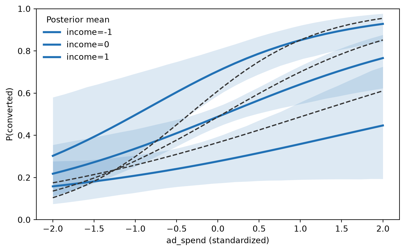

Figure 2: Interventional conversion probability E[converted | do(ad_spend)] vs ad_spend at income=-1,0,1 and segment=1, structural estimator, with 94% HDI bands and planted truth (black dashed).

Response mean vs posterior predictive

predictions() returns kind="mean" draws: expected conversion probability with residual noise off. Posterior predictive bands (sampling 0/1 outcomes) require do(kind="predictive") or sample_posterior_predictive(); this notebook stays on the mean surface that comparisons() and ate() share.

Associational vs interventional

Without set, predictions() evaluates the fitted structural equations at observed covariates. With set, graph surgery fixes ad spend while income follows each row’s profile.

pred_assoc = scm.predictions("converted", newdata=grid.iloc[:3])
pred_int = scm.predictions(
    "converted",
    set={"ad_spend": grid["ad_spend"].iloc[:3].values},
    newdata=grid.iloc[:3],
)
print("associational:", pred_assoc.causal, pred_assoc.interventional)
print("interventional:", pred_int.causal, pred_int.interventional)

associational: False False
interventional: True True

Structural vs adjustment on the same grid

Both estimators expose predictions() with the same signature. When identification holds and both equations are correctly specified, the interventional curves should overlap.

Code

grid_one = pathmc.datagrid(df, ad_spend=dose_grid, income=[0.0], segment=[1.0])
pred_scm = scm.predictions(
    "converted",
    set={"ad_spend": grid_one["ad_spend"].values},
    newdata=grid_one,
)
pred_adj = adj.predictions(
    set={"ad_spend": grid_one["ad_spend"].values},
    newdata=grid_one,
)

fig, ax = plt.subplots(figsize=(FIG_WIDTH, FIG_HEIGHT))
x = grid_one["ad_spend"].values

for result, color, label in [
    (pred_scm, COLOR_STRUCTURAL, "structural"),
    (pred_adj, COLOR_ADJUSTMENT, "adjustment"),
]:
    samples = result.dataset["converted"].stack(sample=("chain", "draw")).values.T
    plot_hdi_line(x, samples, ax, color=color, alpha=0.2, label=label)

ax.plot(
    x,
    true_prob(x, 0.0, 1.0),
    color=COLOR_TRUE,
    linestyle="--",
    linewidth=1.5,
    label="true",
)
ax.set_xlabel("ad_spend")
ax.set_ylabel("P(converted)")
ax.set_ylim(0, 1)
ax.legend(frameon=False)
plt.tight_layout()
plt.show()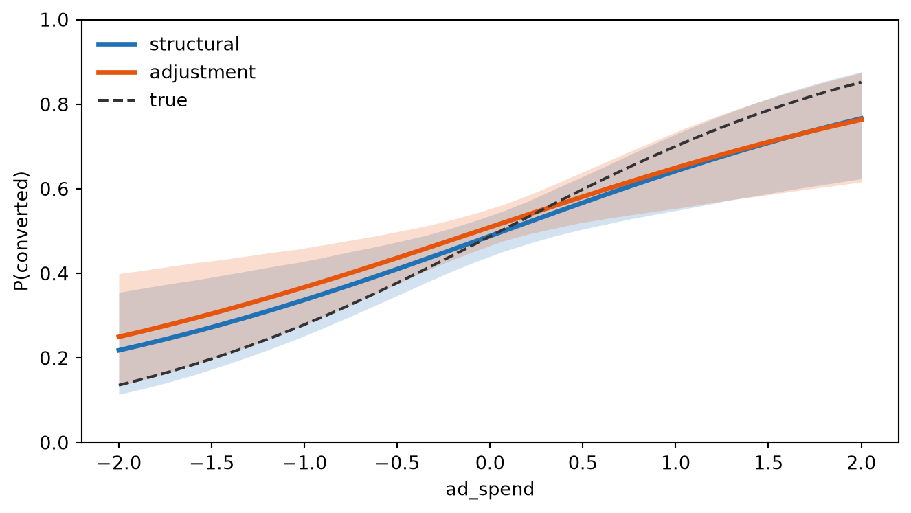

Figure 3: Interventional conversion probability vs ad_spend at income=0 and segment=1: structural g-computation (blue) and regression adjustment (orange), each with 94% HDI; true curve in black dashed.

Customer segment as a categorical covariate

Segment enters the model as a numeric code (0=low, 1=mid, 2=high income tier). On the grid we hold ad spend and income fixed and vary segment; a line plot would be misleading, so we use points with error bars.

Code

seg_grid = pathmc.datagrid(df, ad_spend=[1.0], income=[0.0], segment=[0.0, 1.0, 2.0])
pred_seg = scm.predictions(
    "converted",
    set={"ad_spend": seg_grid["ad_spend"].values},
    newdata=seg_grid,
)
da = pred_seg.dataset["converted"]
means = da.mean(dim=("chain", "draw")).values
stacked = da.stack(sample=("chain", "draw"))
lo = stacked.quantile(0.03, dim="sample").values
hi = stacked.quantile(0.97, dim="sample").values
segments = seg_grid["segment"].values
true_vals = true_prob(1.0, 0.0, segments)

fig, ax = plt.subplots(figsize=(FIG_WIDTH, FIG_HEIGHT))
for i, seg in enumerate(segments):
    color = SEGMENT_COLORS[seg]
    ax.errorbar(
        seg,
        means[i],
        yerr=[[means[i] - lo[i]], [hi[i] - means[i]]],
        fmt="o",
        color=color,
        markersize=8,
        capsize=4,
        linewidth=2,
    )
    ax.plot(
        seg, true_vals[i], marker="D", color=COLOR_TRUE, linestyle="none", markersize=7
    )

ax.set_xticks([0, 1, 2])
ax.set_xticklabels(["low", "mid", "high"])
ax.set_xlabel("segment")
ax.set_ylabel("P(converted)")
ax.set_ylim(0, 1)
plt.tight_layout()
plt.show()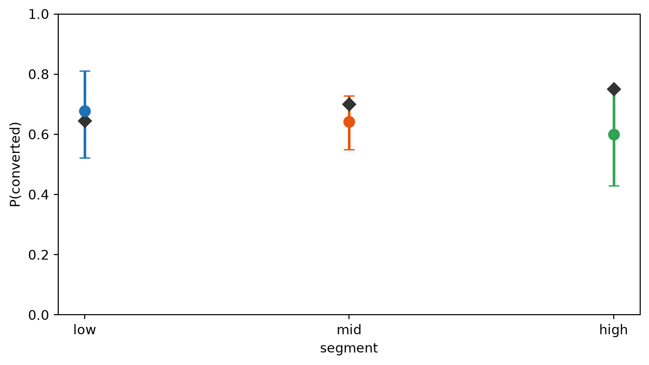

Figure 4: Interventional conversion probability at ad_spend=1, income=0, by customer segment (0=low, 1=mid, 2=high): posterior mean and 94% HDI with true values (black dashed markers).

Predictions table

summary_rows = []
for i in range(len(grid_one)):
    row = grid_one.iloc[i]
    sub = pred_scm.dataset["converted"].isel(unit=i)
    mean = float(sub.mean())
    stacked = sub.stack(sample=("chain", "draw"))
    lo = float(stacked.quantile(0.03))
    hi = float(stacked.quantile(0.97))
    summary_rows.append({
        "ad_spend": row["ad_spend"],
        "income": row["income"],
        "segment": row["segment"],
        "mean": mean,
        "hdi_low": lo,
        "hdi_high": hi,
    })

pd.DataFrame(summary_rows).head(8)

	ad_spend	segment	mean	hdi_low	hdi_high
0	-2.000000	1.0	0.218081	0.113837	0.354866
1	-1.862069	1.0	0.232160	0.127926	0.365269
2	-1.724138	1.0	0.247000	0.143773	0.375374
3	-1.586207	1.0	0.262606	0.160996	0.384457
4	-1.448276	1.0	0.278974	0.180295	0.394634
5	-1.310345	1.0	0.296096	0.200876	0.405140
6	-1.172414	1.0	0.313951	0.222880	0.415911
7	-1.034483	1.0	0.332509	0.245883	0.425727

Summary

datagrid() builds the covariate product; each row is one unit in InterpretResult.
Interventional curves use set={...}; associational baselines omit it (causal=False).
On a Bernoulli outcome the response scale is probability, not log-odds.
Structural and adjustment estimators share the API; overlay them when teaching the two paths.

Next steps: Interventional Contrasts for diff / ratio / lift; Local Slopes when the effect of ad spend depends on income; Predictions, Comparisons, and Slopes for the contract; Causal Inference for ate().

Reflection

In your domain, which covariates belong on a prediction grid (segment, region, product tier) and which are true intervention levers? Would stakeholders read associational fitted curves or only interventional set={...} curves?