Water on a schedule—or when plants need it?
Contrast a fixed irrigation schedule with two stress thresholds on a fitted greenhouse panel, without collapsing posterior or Monte Carlo uncertainty.
A greenhouse can water every third day, or it can water when soil-water stress crosses a threshold. The second rule is a dynamic treatment regime: today’s stress chooses today’s dose, today’s dose changes tomorrow’s stress, and tomorrow’s stress chooses tomorrow’s dose. A schedule copied from the observed stress path, or a threshold applied to the conditional mean of stress, is not that estimand.
The numbers below are a synthetic teaching model, not agronomic advice. Stress is an unbounded standardized index, not a moisture percentage. Irrigation is a binary fixed dose. Heat is external weather. Growth is daily net growth.
Decision, population, and horizon
The decision is which of three rules to follow for the next 30 days: water every third day, water when today’s stress is above 0, or water when today’s stress is above 0.5. Those thresholds were fixed before looking at the policy results. The population is the 12 fitted plots, equally weighted, conditional on the declared pre-sample state and on each plot’s retained heat path. It is not a new-plot forecast. horizon is the fitted day count, 30, and it is passed explicitly.
Data, DGP, and fit
The observational assignment varies with stress, and the growth equation has a stress-by-water interaction, so a responsive rule can matter beyond the total dose. The assignment equation is not fit. The same pre-sample state, stress 0 and water 0, is used in the NumPy generator and in model().
import numpy as np
import pandas as pd
import arviz as az
import matplotlib.pyplot as plt

import pathmc
from pathmc import TimeSchedule, TreatmentPolicy, current, where

N_UNIT = 12
N_TIME = 30
L0 = 0.0
A0 = 0.0
TIMES = list(range(1, N_TIME + 1))
UNITS = [f"plot{i:02d}" for i in range(1, N_UNIT + 1)]

rng = np.random.default_rng(11)
rows = []
for unit in UNITS:
    stress, water = L0, A0
    for time in TIMES:
        heat = float(rng.normal())
        stress = (
            0.4 + 0.6 * stress - 0.8 * water + 0.3 * heat + float(rng.normal(0.0, 0.5))
        )
        prob = 1.0 / (1.0 + np.exp(-(0.2 + 1.2 * stress)))
        water = float(rng.random() < np.clip(prob, 0.1, 0.9))
        growth = (
            1.0
            - 0.6 * stress
            + 0.2 * water
            + 0.6 * stress * water
            + float(rng.normal(0.0, 0.4))
        )
        rows.append({
            "unit": unit,
            "time": time,
            "stress": stress,
            "water": water,
            "heat": heat,
            "growth": growth,
        })
data = pd.DataFrame(rows)
The structural equations are the stress and growth lines of that generator. Water stays an exogenous column: there is no fitted assignment equation, so a posterior predictive of a “natural” watering course is not available and is not invented here.
spec = """
stress ~ lag(stress) + lag(water) + heat
growth ~ stress + water + stress:water
"""
baseline = {"stress": L0, "water": A0}
model = pathmc.model(
    spec,
    data=data,
    panel={"unit": "unit", "time": "time"},
    initial=baseline,
)
idata = model.fit(
    draws=500,
    tune=500,
    chains=4,
    progressbar=False,
    compute_log_likelihood=False,
    random_seed=11,
)
structural = [
    name for name in idata.posterior.data_vars if name.startswith(("beta_", "sigma_"))
]
summary = az.summary(idata, var_names=structural)
print(summary.loc[:, ["mean", "sd", "r_hat", "ess_bulk"]])
assert float(summary["r_hat"].max()) < 1.05
assert float(summary["ess_bulk"].min()) > 400
NUTS[nutpie]: [sigma_stress, beta_growth, beta_stress, carry_innovations_stress, sigma_growth] mean sd r_hat ess_bulk
beta_growth[Intercept] 0.968 0.035 1.00 1728
beta_growth[stress] -0.682 0.047 1.00 1676
beta_growth[water] 0.237 0.046 1.00 1772
beta_growth[stress:water] 0.752 0.061 1.00 2093
beta_stress[Intercept] 0.427 0.04 1.00 2354
beta_stress[lag(stress)] 0.557 0.041 1.00 3412
beta_stress[lag(water)] -0.882 0.058 1.00 2294
beta_stress[heat] 0.294 0.0254 1.01 4008
sigma_stress 0.5125 0.0187 1.00 3497
sigma_growth 0.3838 0.0147 1.00 4978The structural R-hat and bulk ESS are the fit check. Auxiliary innovation coordinates are left out of that check; a warning on those coordinates is not a structural failure. The coefficient table is the observed-data check on the stress and growth equations. Water has no posterior predictive: the assignment equation was not fit, so this page does not invent a natural treatment course.
Three rules, fixed before the results
Water every third day, or when today’s stress is strictly above 0, or strictly above 0.5. All three calls share the posterior, the baseline, the retained heat path, the seed, the horizon, and the simulation count.
every_third = TreatmentPolicy(
    "every_third",
    "water",
    TimeSchedule(tuple(1.0 if i % 3 == 0 else 0.0 for i in range(N_TIME))),
)
threshold_0 = TreatmentPolicy(
    "threshold_0",
    "water",
    where(current("stress") > 0.0, 1.0, 0.0),
)
threshold_05 = TreatmentPolicy(
    "threshold_0.5",
    "water",
    where(current("stress") > 0.5, 1.0, 0.0),
)
shared = dict(
    simulate_over="time",
    horizon=N_TIME,
    initial=baseline,
    n_simulations=64,
    random_seed=11,
)
schedule = model.do(policy=every_third, **shared)
open_rule = model.do(policy=threshold_0, **shared)
tight_rule = model.do(policy=threshold_05, **shared)
Unit traces
One posterior draw and one process replicate, for three plots. The horizontal line is the 0.5 threshold. The action is the executor’s realized dose, not the observed assignment.
traced = model.do(
    policy=threshold_05,
    simulate_over="time",
    horizon=N_TIME,
    initial=baseline,
    n_simulations=4,
    random_seed=11,
    keep_trajectories=True,
)
stress_path = traced.trajectories["stress"].isel(chain=0, draw=0, simulation=0)
water_path = traced.trajectories["water"].isel(chain=0, draw=0, simulation=0)
fig, axes = plt.subplots(2, 1, figsize=(8, 4.5), sharex=True)
for unit in UNITS[:3]:
    axes[0].plot(TIMES, stress_path.sel(unit=unit), label=unit)
    axes[1].step(TIMES, water_path.sel(unit=unit), where="mid", label=unit)
axes[0].axhline(0.5, color="black", linestyle="--", linewidth=1)
axes[0].set_ylabel("stress")
axes[1].set_ylabel("water")
axes[1].set_xlabel("day")
axes[0].legend()
fig.tight_layout()
plt.show()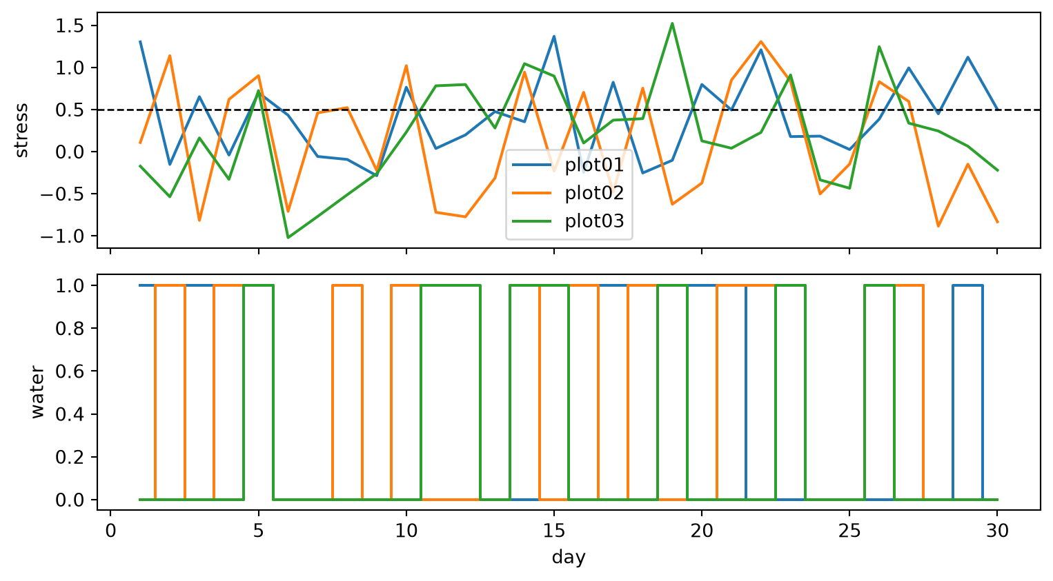
Posterior trajectories and cumulative contrasts
First inspect the posterior mean of each population path. Then subtract the same scheduled baseline from each threshold policy within matching posterior draws and process replicates. Cumulative growth and cumulative water are separate outcomes; their paired contrasts report what changes under each rule.
fig, axes = plt.subplots(1, 2, figsize=(8, 3.5), sharex=True)
for result, label in (
    (schedule, "every third"),
    (open_rule, "threshold 0"),
    (tight_rule, "threshold 0.5"),
):
    axes[0].plot(TIMES, result.by_time("growth").mean(axis=1), label=label)
    axes[1].plot(TIMES, result.by_time("water").mean(axis=1), label=label)
axes[0].set_title("growth")
axes[1].set_title("water")
axes[0].set_xlabel("day")
axes[1].set_xlabel("day")
axes[0].legend()
fig.tight_layout()
plt.show()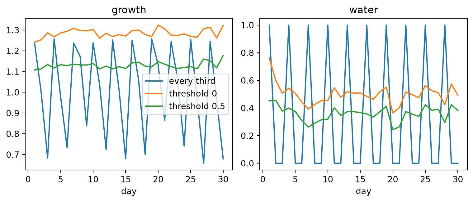
def cumulative(result, var):
    return result.aggregate_time(var, reduction="sum")


for name, result in (
    ("every third", schedule),
    ("threshold 0", open_rule),
    ("threshold 0.5", tight_rule),
):
    growth = cumulative(result, "growth")
    water = cumulative(result, "water")
    print(
        name,
        float(growth.mean("growth")),
        float(water.mean("water")),
        float(np.max(np.abs(growth.simulation_mcse("growth")))),
    )
every third 30.15557708673793 10.0 0.19216025022521943
threshold 0 38.5376836018602 15.006123697916667 0.11549345756255068
threshold 0.5 33.880656673050865 10.768218098958332 0.12949725723997757The following table answers the comparison directly. A positive growth contrast means more cumulative net growth than scheduled watering; a positive water contrast means more fixed doses. The 94% HDI summarizes posterior uncertainty about each expected difference. The maximum per-draw Monte Carlo standard error measures the numerical precision of integrating process noise, separately from that interval.
contrasts = {
    "threshold 0 - schedule": open_rule - schedule,
    "threshold 0.5 - schedule": tight_rule - schedule,
}
contrast_rows = []
for name, contrast in contrasts.items():
    for var in ("growth", "water"):
        total = cumulative(contrast, var)
        lower, upper = total.hdi(var)
        contrast_rows.append({
            "comparison": name,
            "outcome": var,
            "mean difference": total.mean(var),
            "94% HDI lower": lower,
            "94% HDI upper": upper,
            "max per-draw MCSE": float(total.simulation_mcse(var).max()),
        })
contrast_summary = pd.DataFrame(contrast_rows).set_index(["comparison", "outcome"])
contrast_summary.round(3)| mean difference | 94% HDI lower | 94% HDI upper | max per-draw MCSE | ||
|---|---|---|---|---|---|
| comparison | outcome | ||||
| threshold 0 - schedule | growth | 8.382 | 6.452 | 10.293 | 0.148 |
| water | 5.006 | 3.992 | 5.882 | 0.092 | |
| threshold 0.5 - schedule | growth | 3.725 | 1.953 | 5.453 | 0.180 |
| water | 0.768 | -0.352 | 1.911 | 0.090 |
Repeat the paired calculation with another process seed to check numerical stability. Both calls in the repeat share that new seed; subtracting runs with different seeds is rejected.
repeated = {**shared, "random_seed": 29}
repeat = model.do(policy=threshold_05, **repeated)
repeat_schedule = model.do(policy=every_third, **repeated)
first = cumulative(contrasts["threshold 0.5 - schedule"], "growth").mean("growth")
second = cumulative(repeat - repeat_schedule, "growth").mean("growth")
print("paired seed repeat", float(first), float(second), float(abs(first - second)))
paired seed repeat 3.7250795863129333 3.726060166035538 0.0009805797226047908labels = ["every third", "threshold 0", "threshold 0.5"]
results = [schedule, open_rule, tight_rule]
growth_use = [float(cumulative(result, "growth").mean("growth")) for result in results]
water_use = [float(cumulative(result, "water").mean("water")) for result in results]
fig, ax = plt.subplots(figsize=(6, 3.5))
ax.scatter(water_use, growth_use)
for label, x_value, y_value in zip(labels, water_use, growth_use, strict=True):
ax.annotate(label, (x_value, y_value), textcoords="offset points", xytext=(6, 4))
ax.set_xlabel("cumulative water")
ax.set_ylabel("cumulative growth")
fig.tight_layout()
plt.show()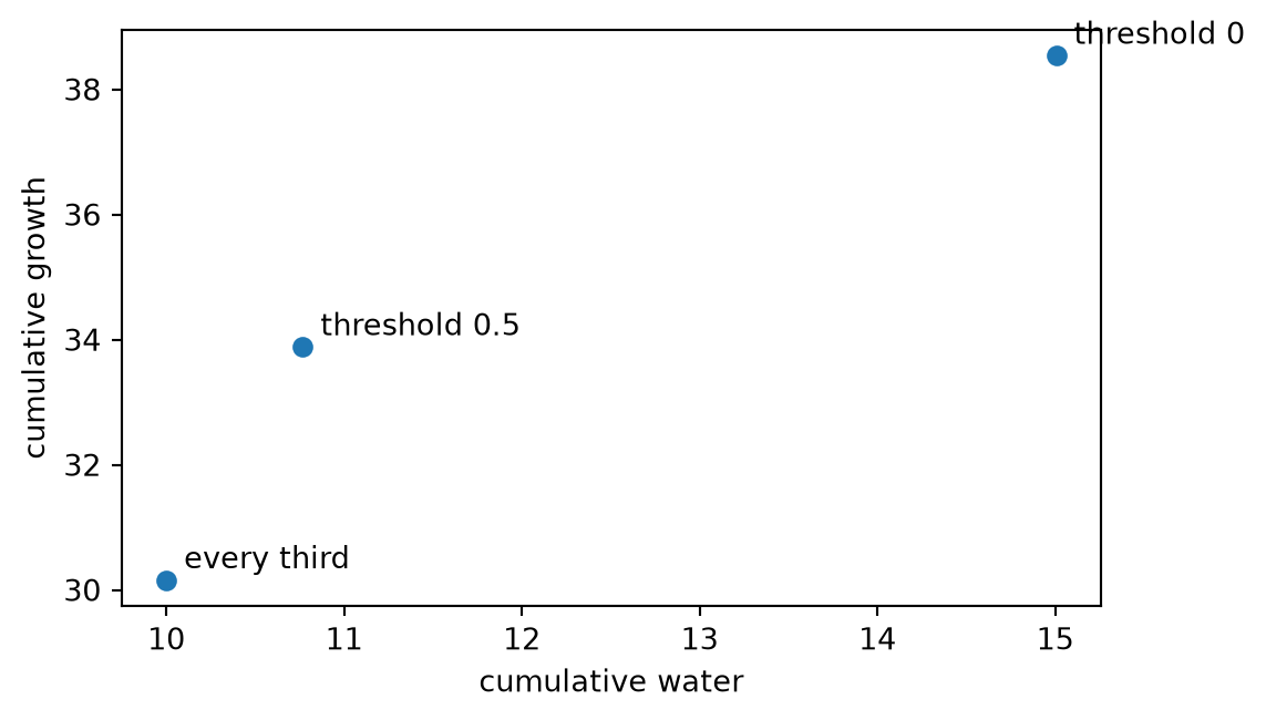
simulation_mcse stays a value per posterior draw. The printed number is the largest absolute per-draw Monte Carlo standard error of cumulative growth, not an average of those standard errors and not the posterior HDI. The second seed is a stability check, not a second estimand. A production contrast should raise n_simulations until that per-draw error is small relative to the contrast of interest.
Two calculations that answer a different question
Thresholding one plot’s observed stress and replaying that dose sequence is a fixed schedule. It does not re-read the stress the policy would have produced. A zero-noise roll of the known generator, with heat fixed at 0, is also not the fitted estimand: the threshold-0.5 path moves when process noise is restored, which is why the policy mean has to integrate the stochastic history.
observed = data[data["unit"] == UNITS[0]].sort_values("time")
copied = TreatmentPolicy(
    "observed_history",
    "water",
    TimeSchedule(tuple(float(value > 0.5) for value in observed["stress"])),
)
copied_result = model.do(policy=copied, **shared)
print(
    "copied schedule growth",
    float(cumulative(copied_result, "growth").mean("growth")),
)
print(
    "threshold 0.5 growth",
    float(cumulative(tight_rule, "growth").mean("growth")),
)


def known_roll(threshold, sigma, n_rep, seed):
    """Known-parameter roll. Heat is fixed at 0. Not the fitted estimand."""
    rng = np.random.default_rng(seed)
    growth = np.zeros(n_rep)
    water_use = np.zeros(n_rep)
    stress = np.full(n_rep, L0)
    water = np.full(n_rep, A0)
    for _ in range(12):
        shock = 0.0 if sigma == 0.0 else rng.normal(0.0, 0.5, size=n_rep)
        stress = 0.4 + 0.6 * stress - 0.8 * water + shock
        action = np.where(stress > threshold, 1.0, 0.0)
        y_shock = 0.0 if sigma == 0.0 else rng.normal(0.0, 0.4, size=n_rep)
        growth += 1.0 - 0.6 * stress + 0.2 * action + 0.6 * stress * action + y_shock
        water_use += action
        water = action
    return float(growth.mean()), float(water_use.mean())


print("zero noise", known_roll(0.0, 0.0, 1, 0), known_roll(0.5, 0.0, 1, 0))
print("with noise", known_roll(0.0, 1.0, 2000, 5), known_roll(0.5, 1.0, 2000, 5))
copied schedule growth 22.880293054554638
threshold 0.5 growth 33.880656673050865
zero noise (14.015808666009601, 6.0) (11.9056503996416, 4.0)
with noise (14.759330812872118, 6.329) (12.970439553921683, 4.365)The zero-noise and noisy known-parameter numbers are exploratory. They are not hard-coded targets for the fitted contrast. The fitted contrast conditions on the observed heat path and on the posterior, which this roll does not.
Assumptions and what this does not support
A causal reading of the contrast needs sequential exchangeability, consistency, treatment support over relevant histories, model adequacy, and no cross-unit interference. Static backdoor checks do not prove longitudinal identification. A marginal min/max warning does not establish sequential positivity: the dose has to be supportable on the stress histories the rule visits, not merely inside the observed stress range.
policy= does not fit an assignment model, optimize a threshold, or accept a Python callback. Latent variables, non-Gaussian families, adstock and other transforms, categoricals, and residual covariance are rejected rather than run on a weaker executor. kind="predictive" is not a noise-free policy mode.