Spline Smooths

Choose among bs(), ns(), and ps() for one curved predictor, and see frozen-knot extrapolation.

A spline is a curve made of polynomial pieces joined at knots. Reach for one when a single predictor is curved and you do not want to commit to a named dose–response formula, estimate its parameters, and hope the form was right. pathmc has three. They are not three names for one smooth.

• bs(dose, df=12) is a cubic B-spline. df is the number of free coefficients, not the number of knots. Each coefficient gets an independent normal prior. Outside the training boundary the curve continues as a cubic.
• ps(dose, df=12) is a P-spline: the same cubic B-spline columns as bs(), plus a random-walk penalty on adjacent coefficients. The default prior penalizes those coefficients, and tau stays at HalfNormal(sigma=2) unless you override it. Outside the training boundary it is the same cubic.
• ns(dose, df=12) is a natural cubic spline. It is unpenalized inside the data and continues as a straight line outside the training boundary. Pass df or knots, not both.

A repeating cycle belongs with fourier(). A smooth that should have a lengthscale and a hard support boundary belongs with hsgp(). The basis-terms guide is the contract for the syntax, the owned coefficients, and the limits. This page is the choice among the three calls.

A curve that is still rising

The true mean below is a logistic dose–response. It starts near 0.3, is halfway through its rise at dose 36, and would flatten near 2.2 if the doses continued. The observations stop at 40, while the curve is still rising, so a line through the last slope is not the plateau. Noise has standard deviation 0.35, large enough that an unpenalized basis with more coefficients than this curve needs will follow it.

import warnings

import arviz as az
import matplotlib.pyplot as plt
import numpy as np
import pandas as pd

import pathmc

FIG_WIDTH = 8
FIG_HEIGHT = 3.6
COLOR_OBSERVED = "#4c78a8"
COLOR_BS = "#e45756"
COLOR_PS = "#f58518"
COLOR_NS = "#b279a2"
COLOR_TRUE = "black"
COLOR_MARK = "0.45"

# Free coefficients, not interior knots. The three calls below share this.
df_spline = 12


def response_mean(x):
    """Logistic still rising at the last observed dose."""
    z = (np.asarray(x, dtype=float) / 36.0) ** 6
    return 0.3 + 1.9 * z / (1.0 + z)


rng = np.random.default_rng(1)
dose = np.linspace(0.0, 40.0, 60)
df = pd.DataFrame({
    "dose": dose,
    "response": response_mean(dose) + rng.normal(0.0, 0.35, size=dose.size),
})

fig, ax = plt.subplots(figsize=(FIG_WIDTH, FIG_HEIGHT))
ax.scatter(
    df["dose"],
    df["response"],
    s=16,
    alpha=0.55,
    color=COLOR_OBSERVED,
    label="Observed",
)
ax.plot(
    dose,
    response_mean(dose),
    color=COLOR_TRUE,
    ls="--",
    lw=1.5,
    label="True mean",
)
ax.set(xlabel="Dose (arbitrary units)", ylabel="Response (arbitrary units)")
ax.legend()
plt.show()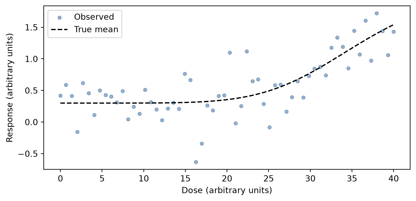

Figure 1: Simulated dose–response on doses 0 to 40. Points include observation noise; the dashed curve is the true mean, still rising at the last dose.

bs() and ps(): same columns, different prior

The next two fits use the same columns. The prior is the only difference, so this is where the penalty earns its place.

model_ps = pathmc.model(f"response ~ ps(dose, df={df_spline})", data=df)
model_ps.equations(show="structural")

\begin{aligned} \mu_{response} &= \beta_{0,\,response} + \operatorname{ps}(\mathrm{dose}) \\ \mathrm{response} &\sim \text{Normal}(\mu_{response},\, \sigma_{response}) \end{aligned}

The rendered equation has no coefficient prefix, and it does not display df. df_spline counts free coefficients, not interior knots. Pass df or knots, not both. The columns are centered, so the intercept remains the mean response. A prefix such as b*ps(dose, df=12) is rejected, because the spline carries its own weights. The guide covers 0 +, panel and endogenous inputs, and self-products.

bs() puts an independent Normal(0, 10) on every coefficient. You chose df_spline, and that is the complexity: extra coefficients are free to follow the noise.

ps() maps a random walk onto those same coefficients. The default order=2 leaves two directions unpenalized, the level and the slope, each at scale 10. Every later coefficient is a unit-scale innovation, and tau multiplies only those. The default for tau is HalfNormal(sigma=2). You can override it. This page does not.

priors() prints that innovation scale as one NumPy vector: 10. twice, then 1. for the rest. The math renderer does not parse the brackets, so the decimal points look like separators between separate priors. They are not. The split is the one just stated, and tau_ps_response_dose is the penalty scale.

model_bs = pathmc.model(f"response ~ bs(dose, df={df_spline})", data=df)
idata_bs = model_bs.fit(draws=800, tune=800, chains=4, random_seed=1)
idata_ps = model_ps.fit(draws=800, tune=800, chains=4, random_seed=1)

NUTS[nutpie]: [beta_bs_response_dose, beta_response, sigma_response]

NUTS[nutpie]: [beta_ps_response_dose, tau_ps_response_dose, beta_response, sigma_response]

# Knots are frozen at fit. No public accessor returns them.
bs_state = model_bs._pymc_model._pathmc_basis_states[("response", "bs", "dose", None)]
ps_state = model_ps._pymc_model._pathmc_basis_states[("response", "ps", "dose", None)]
stored_knots = ps_state.interior
assert stored_knots == bs_state.interior
assert ps_state.boundary == (float(dose.min()), float(dose.max()))

def _mean_hdi(posterior):
    draws = posterior.stack(sample=("chain", "draw")).transpose("sample", ...).values
    return draws.mean(axis=0), az.hdi(draws, prob=0.94, axis=0)


bs_mean, bs_hdi = _mean_hdi(idata_bs.posterior["mu_response"])
ps_mean, ps_hdi = _mean_hdi(idata_ps.posterior["mu_response"])
truth_on_dose = response_mean(dose)
bs_gap = float(np.mean(np.abs(bs_mean - truth_on_dose)))
ps_gap = float(np.mean(np.abs(ps_mean - truth_on_dose)))
bs_rough = float(np.mean(np.abs(np.diff(bs_mean, n=2))))
ps_rough = float(np.mean(np.abs(np.diff(ps_mean, n=2))))
assert ps_gap < bs_gap
assert bs_rough > ps_rough

fig, ax = plt.subplots(figsize=(FIG_WIDTH, FIG_HEIGHT))
ax.scatter(
    df["dose"],
    df["response"],
    s=16,
    alpha=0.35,
    color=COLOR_OBSERVED,
    label="Observed",
    zorder=1,
)
ax.fill_between(
    dose,
    bs_hdi[:, 0],
    bs_hdi[:, 1],
    color=COLOR_BS,
    alpha=0.2,
    label="bs 94% HDI",
)
ax.fill_between(
    dose,
    ps_hdi[:, 0],
    ps_hdi[:, 1],
    color=COLOR_PS,
    alpha=0.2,
    label="ps 94% HDI",
)
ax.plot(dose, bs_mean, color=COLOR_BS, lw=2.2, label="bs posterior mean", zorder=3)
ax.plot(dose, ps_mean, color=COLOR_PS, lw=2.2, label="ps posterior mean", zorder=4)
ax.plot(
    dose,
    truth_on_dose,
    color=COLOR_TRUE,
    ls="--",
    lw=1.5,
    label="True mean",
    zorder=2,
)
ax.set(xlabel="Dose (arbitrary units)", ylabel="Response (arbitrary units)")
ax.legend(fontsize=8, ncol=2)
plt.show()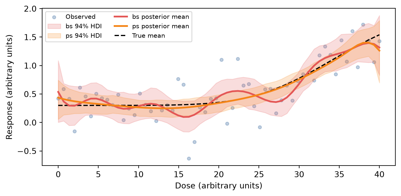

Figure 2: Posterior means of the response for bs() and ps() at the same df, each with a 94% HDI. The dashed curve is the true mean.

The red mean keeps the extra wiggle. On average it sits 0.09 from the true mean, against 0.04 for the orange mean. That gap is the penalty spending coefficients the curve does not need. ps() still uses the bs() columns, so a dose past the data is still a cubic. The next section draws that geometry. The ps() tail is on the figure, and it lands on the bs() cubic.

Extrapolation past the observed doses: ns(), bs(), and ps()

Outside the doses the basis was built on, ns() continues as a line and bs() continues as a cubic. ps() uses the bs() columns, so a least-squares fit on those columns is the same cubic. It is drawn as orange markers on the red curve, so that identity is visible. Neither continuation is the plateau the true mean is heading toward.

The boundary is the range of the training doses, not the range of a later grid. Building the call on a grid that already extends past the last dose would move the boundary to that new end. Inside it, the columns are ordinary, and the line-versus-cubic contrast is gone.

ns_model = pathmc.model(
    f"response ~ ns(dose, knots={stored_knots})",
    data=df,
)
ns_model.equations()

\begin{aligned} \beta_{response} &\sim \text{Normal}(mu=0,\, sigma=10) \\ \sigma_{response} &\sim \text{HalfNormal}(sigma=1) \\ \beta_{ns,response,dose} &\sim \text{Normal}(mu=0,\, sigma=10.0) \\[6pt] \mu_{response} &= \beta_{0,\,response} + \operatorname{ns}(\mathrm{dose}) \\ \mathrm{response} &\sim \text{Normal}(\mu_{response},\, \sigma_{response}) \end{aligned}

That equation has no tau. The single coefficient symbol is the vector of free coefficients, not one coefficient, the same way the structural equation above hides df. With these stored knots, ns() has one more coefficient than the knot count. The cubic bs() fit has the knot count plus the degree. ps() has that same count, because the columns are the same. The figure uses the stored knots, so the comparison is the tail rather than a second knot placement.

from pathmc.basis import get_basis
from pathmc.parse import BasisCall

# End past the point where the cubic slope changes sign, and before it leaves
# the response scale. Dose 50 is too early: only the line has left the truth.
TAIL_END = 56.0


def _extended(name, knots):
    """Least squares of the true mean, evaluated on the stored knots."""
    basis = get_basis(name)
    call = BasisCall(name, "dose", {"knots": knots})
    columns, state = basis.build_data(dose, call)
    assert state.boundary == (float(dose.min()), float(dose.max()))
    truth = response_mean(dose)
    beta, *_ = np.linalg.lstsq(columns, truth - truth.mean(), rcond=None)
    grid = np.linspace(20.0, TAIL_END, 200)
    extended, replayed = basis.build_data(grid, call, state=state)
    assert replayed.boundary == state.boundary
    return grid, truth.mean() + extended @ beta


tail_grid, ns_curve = _extended("ns", stored_knots)
_, bs_curve = _extended("bs", stored_knots)
_, ps_curve = _extended("ps", stored_knots)
assert np.allclose(ps_curve, bs_curve)
tail_truth = response_mean(tail_grid)
train_span = float(np.ptp(response_mean(dose)))
tail_ns_gap = abs(ns_curve[-1] - tail_truth[-1]) / train_span
tail_bs_gap = abs(bs_curve[-1] - tail_truth[-1]) / train_span
tail_sep = abs(ns_curve[-1] - bs_curve[-1]) / train_span
assert tail_ns_gap > 0.15
assert tail_bs_gap > 0.15
assert tail_sep > 0.15
assert (
    response_mean(dose).min() - train_span
    < bs_curve[-1]
    < (response_mean(dose).max() + train_span)
)

fig, ax = plt.subplots(figsize=(FIG_WIDTH, FIG_HEIGHT))
ax.plot(
    tail_grid, ns_curve, color=COLOR_NS, lw=2.2, label="ns() least squares", zorder=2
)
ax.plot(
    tail_grid, bs_curve, color=COLOR_BS, lw=2.2, label="bs() least squares", zorder=3
)
ax.plot(
    tail_grid,
    ps_curve,
    color=COLOR_PS,
    ls="none",
    marker="o",
    ms=5,
    markevery=8,
    label="ps() least squares",
    zorder=5,
)
ax.plot(
    tail_grid,
    tail_truth,
    color=COLOR_TRUE,
    ls="--",
    lw=1.8,
    label="True mean",
    zorder=4,
)
ax.axvline(40.0, color=COLOR_MARK, ls="-", lw=1.0, label="Last observed dose")
ax.set(xlabel="Dose (arbitrary units)", ylabel="Response (arbitrary units)")
ax.legend()
plt.show()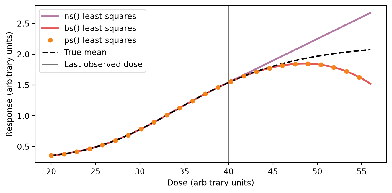

Figure 3: Least-squares fit of the true mean on the training doses, evaluated past the last dose on the knots stored at fit. ns() holds the boundary slope as a line. bs() continues as a cubic and leaves the true flattening. ps() is marked on that same cubic: the columns match, so the least-squares tail matches.

Past the last observed dose the purple curve holds the boundary slope as a line. The red curve bends away from the true flattening: at dose 56 it is 45% of the training span off the true mean, the line is 48% off it, and the two tails are 93% of that span apart. The orange markers are ps(). They are not a third shape. They use the bs() columns, so this least-squares tail is the red cubic. The penalty changes the posterior in the previous figure, not this geometry. The cubic has not found a plateau, and it has not found a peak the data contained. It is the polynomial continuation of the boundary derivatives. Use ns() when a dose past the data should stay on a line. It cannot follow a bend outside the range, and it has no penalty inside.

What do() uses past the last observed dose

You already fit ps() on doses 0 to 40. The question here is the response at a dose past that range. do() answers it: replace the dose column, keep the knots from the fit, and return the posterior mean of the response. A different implementation could see the new doses, place new knots, and answer a different basis than the one you fit. pathmc does not. do() and predict() replay the knots stored at fit. A new dose does not move the basis.

# One value per observed row, from the last dose to just past the boundary.
future_dose = np.linspace(40.0, 42.0, len(df))

future_dose has one value per observed row and runs from 40 to 42, just far enough to leave the training boundary. set={"dose": future_dose} replaces the dose column. kind="mean" asks for the posterior mean of the response at each future dose, the same quantity as the in-sample mu_response. average_units=False keeps one mean per dose. The default True would collapse the grid to one number and hide the continuation.

The printout has three lines. The warning says the dose is outside the observed range. That is all it says. A fresh build on the new grid would warn too. The two numbers are this fit continued: the posterior mean at dose 40 and at dose 42. They are not the red least-squares cubic from the previous figure. This fit is already turning down at the last observed dose, and the call carries that bend with it.

with warnings.catch_warnings(record=True) as caught:
    warnings.simplefilter("always")
    continued = model_ps.do(
        set={"dose": future_dose},
        kind="mean",
        average_units=False,
        random_seed=1,
    )
warning = next(
    item.message for item in caught if issubclass(item.category, UserWarning)
)
unit_means = continued.dataset["response"].mean(("chain", "draw")).values
print(warning)
print(f"posterior mean at dose {future_dose[0]:.0f}: {float(unit_means[0]):.2f}")
print(f"posterior mean at dose {future_dose[-1]:.0f}: {float(unit_means[-1]):.2f}")

Intervention value [40.00, 42.00] for 'dose' is outside the observed data range [0.00, 40.00]. Results are extrapolations and should be interpreted with caution.
posterior mean at dose 40: 1.26
posterior mean at dose 42: 0.49

The warning and the two numbers do not show which knots were used. do() does not return the columns it substituted, and equations() cannot show the stored knots. The next cell repeats the same call. It is folded because it is a probe, not the call you would write. Read the three printed lines. The first tuple is the interior knots stored at fit. The second is what a fresh df_spline build places on these future doses. The number is the largest gap between the columns this call used and that fresh build.

import pathmc.basis as _basis
from pathmc.basis import get_basis
from pathmc.parse import BasisCall

# do() does not return the columns it substituted, and it does not
# write them back. This second call is the same intervention, wrapped
# only so the printed tuples can show the columns it used.
_real_replay = _basis.replay_data_bases
_substituted = {}


def _capture_replay(bindings, values):
    updates = _real_replay(bindings, values)
    _substituted.update(updates)
    return updates


_basis.replay_data_bases = _capture_replay
try:
    with warnings.catch_warnings():
        warnings.simplefilter("ignore", UserWarning)
        model_ps.do(
            set={"dose": future_dose},
            kind="mean",
            average_units=False,
            random_seed=1,
        )
finally:
    _basis.replay_data_bases = _real_replay

_items = [
    (name, binding)
    for name, binding in model_ps._gen_model._pathmc_data_bases.items()
    if binding.call.name == "ps" and binding.call.variable == "dose"
]
assert len(_items) == 1
_data_name, _binding = _items[0]
substituted = _substituted[_data_name]
training_columns, _ = _binding.basis.build_data(
    future_dose, _binding.call, state=_binding.state
)
refit_columns, refit_state = get_basis("ps").build_data(
    future_dose, BasisCall("ps", "dose", {"df": df_spline})
)
assert np.allclose(substituted, training_columns)
assert not np.allclose(substituted, refit_columns)
max_abs_diff = float(np.max(np.abs(substituted - refit_columns)))
print("max_abs_diff_from_refit", round(max_abs_diff, 2))
print("training", tuple(round(float(k), 1) for k in _binding.state.interior))
print("refit", tuple(round(float(k), 1) for k in refit_state.interior))

max_abs_diff_from_refit 3.26
training (4.0, 8.0, 12.0, 16.0, 20.0, 24.0, 28.0, 32.0, 36.0)
refit (40.2, 40.4, 40.6, 40.8, 41.0, 41.2, 41.4, 41.6, 41.8)

The call matched the stored knots, not the fresh placement. Reading the model afterward would not show that, because do() does not write the knots it applied back onto the binding.

The figure is not that result. It is the right edge of the fit the call continues, so the downturn at dose 40 has a picture. That bend belongs to this noisy fit. The red cubic in the tails figure stays with the true mean past dose 40. Drawing the two future doses would look like that cubic-versus-line lesson and is not, so the continuation is not drawn. The printed means are that continuation. The printed tuples are the proof the knots were kept.

fig, ax = plt.subplots(figsize=(FIG_WIDTH, FIG_HEIGHT))
ax.scatter(
    df["dose"],
    df["response"],
    s=14,
    alpha=0.35,
    color=COLOR_OBSERVED,
    label="Observed",
    zorder=1,
)
ax.fill_between(
    dose,
    ps_hdi[:, 0],
    ps_hdi[:, 1],
    color=COLOR_PS,
    alpha=0.25,
    label="94% in-sample HDI",
)
ax.plot(dose, ps_mean, color=COLOR_PS, lw=2.2, label="In-sample mean")
ax.plot(dose, response_mean(dose), color=COLOR_TRUE, ls="--", lw=1.5, label="True mean")
ax.axvline(40.0, color=COLOR_MARK, ls="-", lw=1.0, label="Last observed dose")
ax.set_xlim(28.0, 40.4)
visible = dose >= 28.0
shown = np.concatenate([
    df.loc[df["dose"] >= 28.0, "response"].to_numpy(),
    ps_hdi[visible, 0],
    ps_hdi[visible, 1],
    ps_mean[visible],
    response_mean(dose[visible]),
])
pad = 0.06 * float(np.ptp(shown))
ax.set_ylim(float(shown.min()) - pad, float(shown.max()) + pad)
ax.set(xlabel="Dose (arbitrary units)", ylabel="Response (arbitrary units)")
ax.legend(fontsize=8, ncol=2)
plt.show()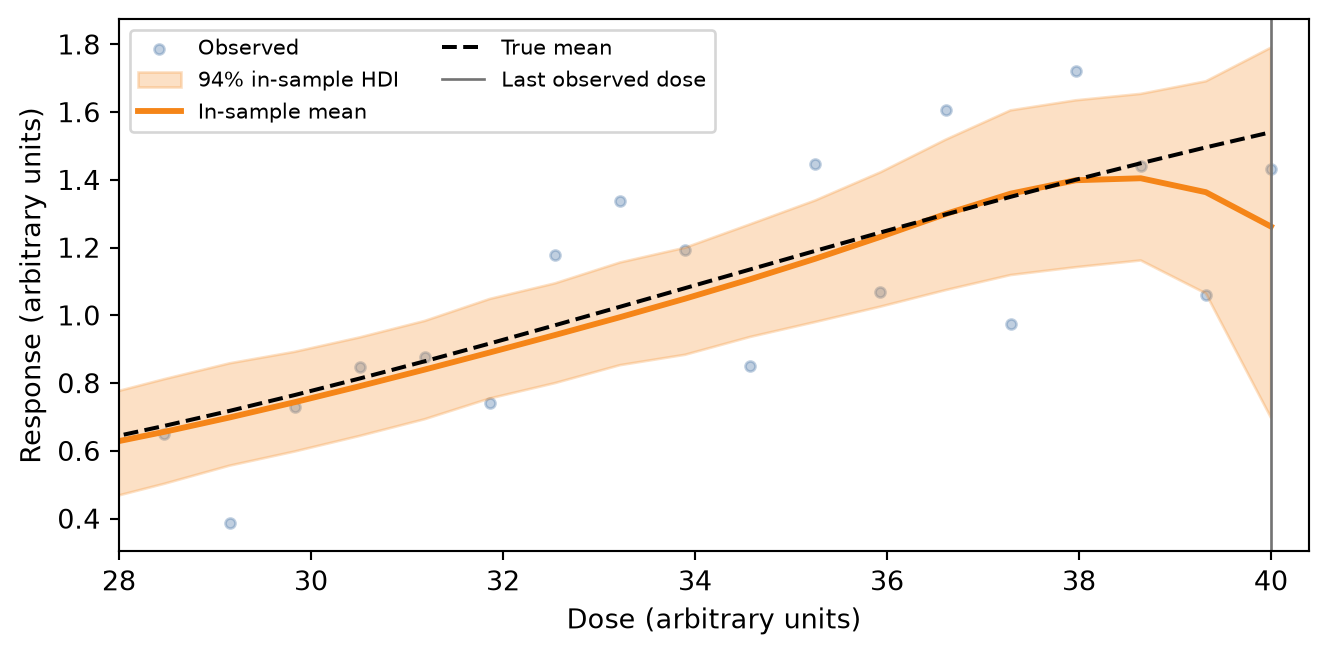

Figure 4: Right edge of the in-sample ps() posterior mean, with a 94% HDI. The mean is already turning down at the last observed dose. That bend is this fit, not the least-squares cubic in the tails figure. The do() continuation is the printed means, not a curve on this figure. The dashed curve is the true mean.

predict() applies the same stored state. It does not emit the extrapolation warning, and it is not plotted.

Choosing

The figures are one curve. The choice is which behavior you want, not which call sits closer to a plateau.

Situation	Call
The extra coefficients should be spent by a penalty, and a cubic continuation past the data is acceptable	ps()
A dose past the data should stay on a straight line	ns()
An unpenalized basis, and you will set df or the coefficient prior yourself	bs()
A lengthscale and a hard support boundary	hsgp()
A pattern that repeats	fourier()

Takeaway: use ps() when a penalty should spend the extra coefficients and a cubic continuation is acceptable, ns() when a dose past the data should stay on a line, and bs() when you will set df or the coefficient prior yourself. The knots stored at fit are what do() and predict() apply to a new dose. Neither the cubic nor the line is the plateau a dose–response may be heading toward.