Nonparametric Smooths with HSGP

Fit a flexible 1-D nonparametric smooth with the hsgp() term — a Hilbert Space Gaussian Process approximation — and predict beyond the observed range with do().

Author

Juan Orduz

Most pathmc terms are linear in their coefficients. A dose–response curve often is not: it can rise, flatten, and still have a local shoulder that no straight line and no single sine wave will follow. The hsgp() term adds that kind of smooth via a Hilbert Space Gaussian Process approximation (Riutort-Mayol et al. 2023), the same scalable construction exposed by Bambi’s hsgp(). It is one of pathmc’s basis terms, alongside fourier() seasonality.

An HSGP approximates a Gaussian process with a finite basis of Laplacian eigenfunctions, so it reduces to a linear model in a fixed basis matrix. That makes it fast, differentiable, and — because the basis is a deterministic function of the input pm.Data — fully compatible with do() interventions.

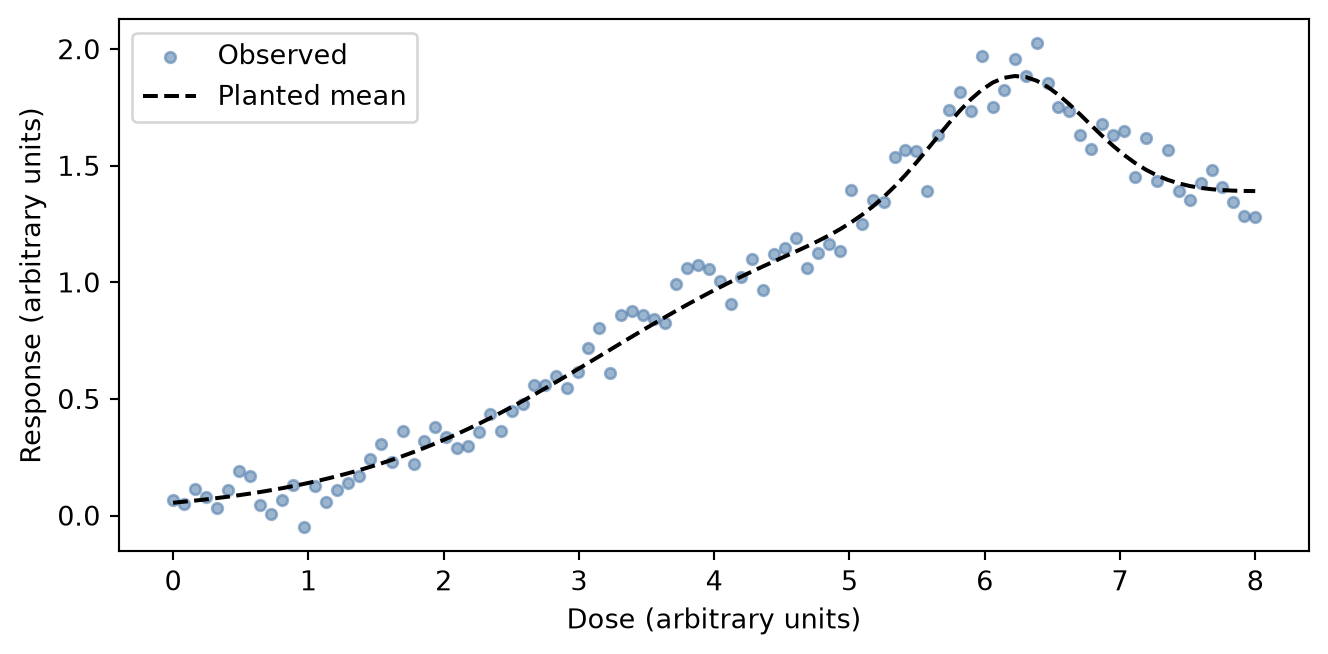
Simulated dose–response

The planted mean is a saturating rise plus a narrow shoulder. Observation noise has standard deviation 0.08. The doses sit on a range of several units, which matters for the lengthscale prior below.

Code

import arviz as az
import matplotlib.pyplot as plt
import numpy as np
import pandas as pd

import pathmc
from pathmc import Prior

FIG_WIDTH = 8
FIG_HEIGHT = 3.6
COLOR_OBSERVED = "#4c78a8"
COLOR_POSTERIOR = "#f58518"
COLOR_FUTURE = "#54a24b"
COLOR_TRUE = "black"


def response_mean(x):
    """Saturating rise plus a narrow shoulder, in response units."""
    rise = 1.4 / (1.0 + np.exp(-(x - 3.2)))
    shoulder = 0.55 * np.exp(-0.5 * ((x - 6.2) / 0.55) ** 2)
    return rise + shoulder


rng = np.random.default_rng(0)
dose = np.linspace(0.0, 8.0, 100)
df = pd.DataFrame({
    "dose": dose,
    "response": response_mean(dose) + rng.normal(0.0, 0.08, size=dose.size),
})

fig, ax = plt.subplots(figsize=(FIG_WIDTH, FIG_HEIGHT))
ax.scatter(
    df["dose"], df["response"], s=16, alpha=0.55, color=COLOR_OBSERVED, label="Observed"
)
ax.plot(
    df["dose"],
    response_mean(dose),
    color=COLOR_TRUE,
    ls="--",
    lw=1.5,
    label="Planted mean",
)
ax.set(xlabel="Dose (arbitrary units)", ylabel="Response (arbitrary units)")
ax.legend()
plt.show()

Figure 1: Simulated dose–response. Points include Gaussian observation noise; the dashed curve is the planted mean, a saturating rise plus a shoulder.

A linear term would miss the plateau, and a single Fourier harmonic would force the shoulder to repeat. The smooth below does not assume either shape.

The model

hsgp(dose, m=..., c=...) is a standalone term: m sets the number of basis vectors and c the boundary-expansion factor. The smooth carries its own basis weights, so it takes no coefficient prefix.

model = pathmc.model("response ~ hsgp(dose, m=20, c=1.5)", data=df)
model.equations()

\begin{aligned} \beta_{response} &\sim \text{Normal}(mu=0,\, sigma=10) \\ \sigma_{response} &\sim \text{HalfNormal}(sigma=1) \\ \ell_{response,dose} &\sim \text{InverseGamma}(alpha=3,\, beta=8.0) \\ \eta_{response,dose} &\sim \text{HalfNormal}(sigma=1) \\ \beta_{hsgp,response,dose} &\sim \text{Normal}(mu=0,\, sigma=1) \\[6pt] \mu_{response} &= \beta_{0,\,response} + f_{\mathrm{hsgp}}(\mathrm{dose}) \\ \mathrm{response} &\sim \text{Normal}(\mu_{response},\, \sigma_{response}) \end{aligned}

The default priors expose the kernel amplitude (eta_response_dose), lengthscale (ell_response_dose), and standardized basis weights (beta_hsgp_response_dose):

model.priors()

The lengthscale prior matches the compiled input column. With data, the default is InverseGamma(3, beta) where beta is that column’s span, so the mean is half the span. This page does not scale dose, so the span is the raw range 0 to 8 and the default mean is 4. Channel scaling rewrites the column before the prior is built, and beta then matches the internal span, not the business-unit range. The cell below tightens the prior to a mean of 2 dose units. Even with that prior, this posterior still diverges at the default target acceptance, because the lengthscale and the basis weights trade off. target_accept=0.99 is the setting that samples it cleanly.

# Mean lengthscale of 2 dose units: InverseGamma(3, 4) has mean 4 / (3 - 1).
model.set_priors({"ell_response_dose": Prior("InverseGamma", alpha=3, beta=4)})

Fit and recover the smooth

idata = model.fit(random_seed=0, target_accept=0.99)

NUTS[nutpie]: [eta_response_dose, ell_response_dose, beta_hsgp_response_dose, beta_response, sigma_response]

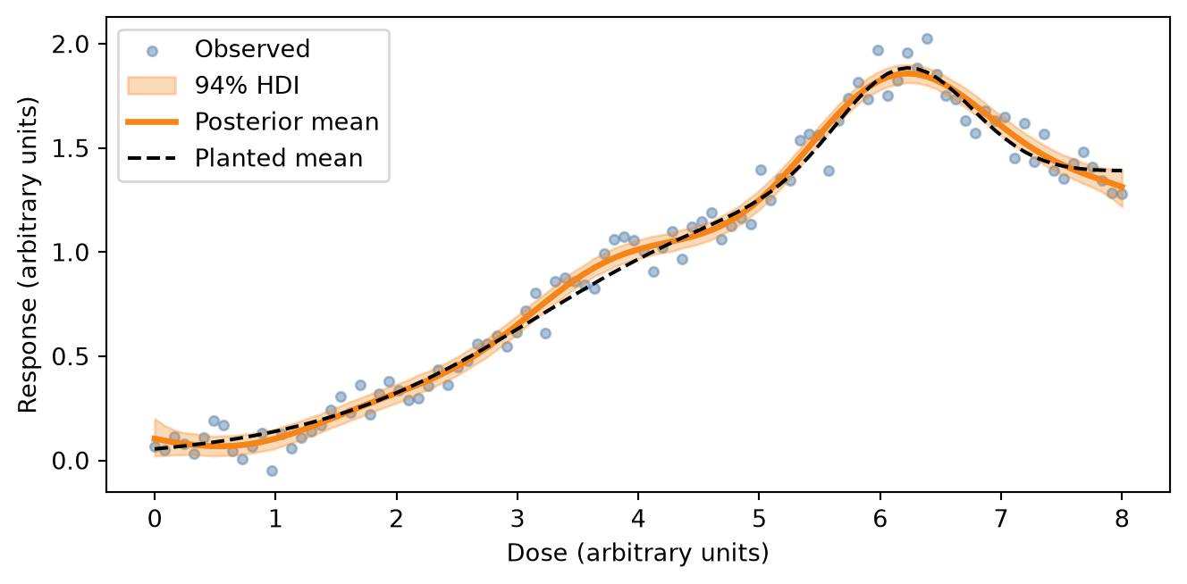
The posterior of mu_response is the full linear predictor, intercept included. The figure shows its mean and 94% highest-density interval against the planted curve, rather than a single point-estimate line.

Code

mu = idata.posterior["mu_response"]
mu_draws = mu.stack(sample=("chain", "draw")).transpose("sample", ...).values
mu_mean = mu_draws.mean(axis=0)
mu_hdi = az.hdi(mu_draws, prob=0.94, axis=0)

fig, ax = plt.subplots(figsize=(FIG_WIDTH, FIG_HEIGHT))
ax.scatter(
    df["dose"],
    df["response"],
    s=16,
    alpha=0.45,
    color=COLOR_OBSERVED,
    label="Observed",
    zorder=1,
)
ax.fill_between(
    dose,
    mu_hdi[:, 0],
    mu_hdi[:, 1],
    color=COLOR_POSTERIOR,
    alpha=0.3,
    label="94% HDI",
    zorder=2,
)
ax.plot(dose, mu_mean, color=COLOR_POSTERIOR, lw=2.5, label="Posterior mean", zorder=3)
ax.plot(
    dose,
    response_mean(dose),
    color=COLOR_TRUE,
    ls="--",
    lw=1.5,
    label="Planted mean",
    zorder=4,
)
ax.set(xlabel="Dose (arbitrary units)", ylabel="Response (arbitrary units)")
ax.legend()
plt.show()

Figure 2: In-sample posterior mean of the response with a 94% HDI. The dashed curve is the planted dose–response; the band covers it across the observed doses.

The posterior mean follows the rise, the plateau, and the shoulder. That is the check that the basis is flexible enough for a curve that is not a sine wave.

Predict past the observed doses

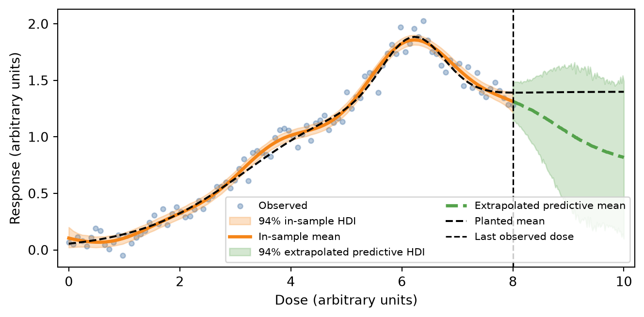
Because the basis recomputes from the input data node, do() propagates through the smooth. With c = 1.5 the basis boundary is wider than the observed doses: the midpoint of [0, 8] is 4 and the half-range is 4, so L = 1.5 × 4 = 6 and the boundary is [−2, 10]. do() replaces the dose column, so the new grid has to have one value per observed row. A grid of the same length running from 8 to 10 sits outside the sample and inside that boundary.

future_dose = np.linspace(8.0, 10.0, len(df))
future = model.do(set={"dose": future_dose}, kind="predictive")

/var/folders/r0/nf1kgxsx6zx3rw16xc3wnnzr0000gn/T/ipykernel_17253/2184046133.py:2: UserWarning: Intervention value [8.00, 10.00] for 'dose' is outside the observed data range [0.00, 8.00]. Results are extrapolations and should be interpreted with caution.
  future = model.do(set={"dose": future_dose}, kind="predictive")
Sampling: [response]

That call warns once: the new doses sit outside the observed range, so the result is an extrapolation. The warning is the right context. The basis is still defined here because 10 is the edge of the boundary, not past it. kind="predictive" includes uncertainty in the smooth and residual noise, so the future band is a posterior predictive interval rather than a noise-free mean curve.

Code

future_draws = future.dataset["response"].values.reshape(-1, future_dose.size)
future_mean = future_draws.mean(axis=0)

future_hdi = az.hdi(future_draws, prob=0.94, axis=0)

fig, ax = plt.subplots(figsize=(FIG_WIDTH, FIG_HEIGHT))
ax.scatter(
    df["dose"],
    df["response"],
    s=14,
    alpha=0.4,
    color=COLOR_OBSERVED,
    label="Observed",
    zorder=1,
)
ax.fill_between(
    dose,
    mu_hdi[:, 0],
    mu_hdi[:, 1],
    color=COLOR_POSTERIOR,
    alpha=0.25,
    label="94% in-sample HDI",
    zorder=2,
)
ax.plot(dose, mu_mean, color=COLOR_POSTERIOR, lw=2.5, label="In-sample mean", zorder=3)
ax.fill_between(
    future_dose,
    future_hdi[:, 0],
    future_hdi[:, 1],
    color=COLOR_FUTURE,
    alpha=0.25,
    label="94% extrapolated predictive HDI",
    zorder=2,
)
ax.plot(
    future_dose,
    future_mean,
    color=COLOR_FUTURE,
    lw=2.5,
    ls="--",
    label="Extrapolated predictive mean",
    zorder=3,
)
extended = np.concatenate([dose, future_dose])
ax.plot(
    extended,
    response_mean(extended),
    color=COLOR_TRUE,
    ls="--",
    lw=1.5,
    label="Planted mean",
    zorder=4,
)
ax.axvline(8.0, color=COLOR_TRUE, ls="--", lw=1.2, label="Last observed dose", zorder=5)
ax.set(
    xlabel="Dose (arbitrary units)",
    ylabel="Response (arbitrary units)",
    xlim=(-0.2, 10.2),
)
ax.legend(fontsize=8, ncol=2)
plt.show()

Figure 3: In-sample posterior mean (orange) and extrapolated posterior predictive mean (green), each with a 94% HDI. The vertical line is the last observed dose. The dashed curve is the planted mean, extended through the extrapolation window.

The green band is wider than the orange one. The basis still has a defined shape on [8, 10], but those doses were not in the likelihood, so the posterior of the smooth is less pinned down. That widening is the honest uncertainty, not a failure of do().

Past the boundary the sinusoidal eigenfunctions alias rather than extrapolate, so do() raises ValueError instead of returning a plausible-looking number. Dose 12 sits beyond 10:

try:
    model.do(set={"dose": 12.0})
except ValueError as err:
    print(err)

Intervention value 12.00 for 'dose' is outside the HSGP basis boundary [-2.00, 10.00] frozen from the fitted data. Beyond this boundary the basis eigenfunctions alias, so the result would be meaningless rather than an extrapolation. Refit with a larger c or an explicit L to widen the valid region.

Scope

Phase 1 supports a single 1-D exogenous input on cross-sectional models. Multi-dimensional inputs, grouped (by=) GPs, and panel/scan models raise a clear error and are tracked as follow-ups.

The input must be exogenous because the basis is built by evaluating it: PyMC derives the centering midpoint and the boundary from the input’s realized values. Smoothing an endogenous variable (one that is itself the outcome of another equation) would freeze the basis at a random prior draw, so pathmc rejects it rather than fitting a model whose result depends on compilation-time RNG.

Takeaway: use hsgp() for a smooth that should not be forced into a line or a repeating cycle, set the lengthscale prior on the scale of the compiled input, and use do() to read the curve past the observed range but inside the basis boundary. For a pattern that repeats, see Fourier seasonality.

References

Riutort-Mayol, Gabriel, Paul-Christian Bürkner, Michael R. Andersen, Arno Solin, and Aki Vehtari. 2023. “Practical Hilbert Space Approximate Bayesian Gaussian Processes for Probabilistic Programming.” Statistics and Computing 33: 17. https://doi.org/10.1007/s11222-022-10167-2.