import numpy as np
import pandas as pd
import pathmc
rng = np.random.default_rng(42)
n = 500
X = rng.normal(size=n)
M = 0.5 * X + rng.normal(scale=0.5, size=n)
Y = 0.8 * M + 0.3 * X + rng.normal(scale=0.5, size=n)
df = pd.DataFrame({"X": X, "M": M, "Y": Y})
spec = """
M ~ a*X
Y ~ b*M + c*X
indirect := a*b
"""
m = pathmc.model(spec, data=df)Welcome


Structural causal models, made simple.
Specify your causal assumptions as equations. Fit with full Bayesian inference. Simulate interventions and ask “what if?”
pathmc compiles a concise formula language into a generative Bayesian model where every variable is wired through its structural parents in the DAG. Call model() to build and inspect, then fit() to run MCMC. One object handles estimation, introspection, causal queries, identification checking, native regression adjustment, and sensitivity analysis, all with full posterior uncertainty.
import pathmc

spec = """
M ~ a*X
Y ~ b*M + c*X
indirect := a*b
"""

m = pathmc.model(spec, data=df)
m.fit(draws=1000, chains=2)

m.effects_summary()  # labeled coefficients + defined params
m.ate("Y", "X", values=(0, 1))  # average treatment effect via do-operator
m.adjustment_sets("X", "Y")  # check identification from the DAG
m.comparisons("Y", "X")  # interpret-layer contrast (diff, or ratio/lift)

adj = m.adjustment_model("X -> Y")  # backdoor-adjusted outcome regression
adj.fit()
adj.ate(values=(0, 1))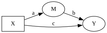
\begin{aligned} \beta_{M} &\sim \text{Normal}(mu=0,\, sigma=10) \\ \sigma_{M} &\sim \text{HalfNormal}(sigma=1) \\ \beta_{Y} &\sim \text{Normal}(mu=0,\, sigma=10) \\ \sigma_{Y} &\sim \text{HalfNormal}(sigma=1) \\[6pt] \mu_{M} &= \beta_{0,\,M} + a \cdot \mathrm{X} \\ \mathrm{M} &\sim \text{Normal}(\mu_{M},\, \sigma_{M}) \\ \mu_{Y} &= \beta_{0,\,Y} + b \cdot \mathrm{M} + c \cdot \mathrm{X} \\ \mathrm{Y} &\sim \text{Normal}(\mu_{Y},\, \sigma_{Y}) \\ indirect &\equiv a \cdot b \end{aligned}
Explore the DAG before you have data
You don’t need a DataFrame to start thinking causally. Pass just a spec string to model() and immediately explore the DAG structure, check identification, and review priors — all before collecting or cleaning data.
m = pathmc.model("""
    M ~ a*X
    Y ~ b*M + c*X
    indirect := a*b
""")

m.graph()  # render the causal DAG
m.equations()  # structural equations + priors
m.adjustment_sets("X", "Y")  # valid backdoor adjustment sets
m.is_identifiable("X", "Y")  # identification check
When data arrives, create a data-bound model and fit:
m = pathmc.model(spec, data=df)
m.fit(draws=1000)
One spec, six capabilities
A single spec string unlocks the full causal analysis toolkit.
Introspection — inspect the model before spending any time on MCMC. Render the causal DAG, display structural equations with LaTeX, review default priors, and refine priors iteratively. graph(), equations(), and set_priors() work with or without data; sample_prior_predictive() requires a data-bound model to set sample size and exogenous inputs.
m.graph()  # causal DAG plot
m.equations()  # structural equations + priors
m.set_priors({"beta_Y": Prior(...)})  # refine priors
m.sample_prior_predictive()  # check priors generate plausible data (requires data)
Estimation — fit the structural model with MCMC. Get posterior summaries, labeled coefficients with uncertainty, path-specific effects, and stdyx-standardized coefficients for comparing effect sizes across variables on different scales.
m.fit()
m.effects_summary()  # labeled coefficients + defined params
m.standardized()  # stdyx-standardized effects
m.effect("X -> M -> Y")  # indirect effect through M
Causal queries — simulate interventions via the do-operator and ask counterfactual questions. pathmc uses g-computation: it forward-simulates through the structural model under the intervention, propagating full posterior uncertainty through the causal chain. The shared interpret layer (predictions(), comparisons(), slopes()) generalizes two-point ate() to grids, ratio/lift contrasts, and local derivatives.
m.ate("Y", "X", values=(0, 1))  # average treatment effect
m.cate("Y", "X", condition={"Z": 2})  # conditional ATE given Z=2
m.prob("Y > 0", set={"X": 1})  # P(Y > 0) under intervention
m.comparisons("Y", "X", comparison="lift")  # percent change on the response scale
m.slopes("Y", "X")  # local derivative under intervention
Identification — before trusting a causal estimate, verify it is identifiable. pathmc finds valid adjustment sets, checks for collider bias, and tests the DAG’s conditional independence claims against your data. Structural checks work without data; test_implications() requires data.
m.adjustment_sets("X", "Y")  # valid backdoor adjustment sets
m.collider_warnings({"C"}, "X", "Y")
m.test_implications()  # check DAG against data
Regression adjustment — when the question is the total effect of one treatment on one outcome, adjustment_model() uses the DAG only for identification, then fits a single reduced outcome equation and standardizes predictions. Same ate() / comparisons() / slopes() names as the structural model. See Estimation Approaches and SCM vs Regression Adjustment.
adj = m.adjustment_model("X -> Y")
adj.formula  # e.g. "Y ~ X + Z"
adj.fit()
adj.ate(values=(0, 1))
adj.comparisons(comparison="diff")
Sensitivity analysis — causal conclusions rest on untestable assumptions about unmeasured confounding. pathmc quantifies how strong an unmeasured confounder would need to be to overturn your finding.
m.sensitivity("Y", "X") # tipping point analysisApplied use cases
pathmc isn’t just for textbook examples. The examples gallery covers real problems across industries.
Estimate channel-level ROI with adstock and saturation transforms that capture carry-over effects and diminishing returns. Panel mode handles geo-level data with hierarchical random effects. Full example →
spec = """
sales ~ b_tv*logistic_saturation(adstock(tv, decay=theta_tv), lam=lam_tv)
      + b_dig*logistic_saturation(adstock(digital, decay=theta_dig), lam=lam_dig)
      + trend
"""
adstock(x, decay=param) models carry-over effects; logistic_saturation(x, lam=param) captures diminishing returns. Both transform parameters are estimated from data alongside the regression coefficients.
Assess whether a biomarker is a valid surrogate for clinical outcomes using mediation analysis and the do-operator. Quantify what fraction of the treatment effect flows through the measured pathway. Full example →
spec = """
antibody     ~ a*vaccine + age
hospitalized ~ b*antibody + c*vaccine + age + comorbidity
"""
Labeled coefficients (a*, b*, c*) let you decompose the total effect into indirect (a*b, through antibodies) and direct (c, bypassing antibodies) pathways.
Model a multi-stage funnel as a causal chain to find which stage has the highest leverage on paid conversion. Simulate “what if we improve onboarding?” scenarios that respect the full causal structure. Full example →
spec = """
engagement ~ e_ch*channel_quality + e_on*onboarding_score
activated  ~ a_eng*engagement + a_ch*channel_quality
converted  ~ c_act*activated + c_eng*engagement
"""
Each equation models one stage. Multiple equations form the causal chain — effects propagate through the system, so improving onboarding lifts engagement, which lifts activation, which lifts conversion.
Estimate true price elasticity from observational data where price and demand are confounded. Panel structure with regional hierarchical effects separates the causal signal from common-cause noise. Full example →
spec = """
demand ~ b_price*price + b_lag*lag(price)
       + b_comp*competitor_price + b_season*season + trend
"""
lag(price) creates the previous period’s value automatically in panel mode. Random slopes on price (specified at model() time) let each region have its own elasticity, partially pooled toward a population mean.
Built-in guardrails
pathmc doesn’t just compute causal effects — it helps you check whether you should trust them.
- Identification checks verify that your causal effect is estimable from observational data before you spend time sampling.
- Collider warnings flag adjustment sets that would create spurious associations rather than remove them.
- Implied independence tests check the conditional independence claims encoded in your DAG against the data — violations suggest missing edges or structural misspecification.
- Sensitivity analysis quantifies how robust your conclusions are to unmeasured confounding, reporting tipping points and contour plots.
The goal is responsible causal inference: make it easy to ask hard questions about your own assumptions.
Getting started
- Overview — how pathmc works, from spec to causal insight
- Bayesian workflow — the iterative cycle of inspect, check, refine, fit, and query
- Model specification — DSL syntax:
~,~~,:=, labels, transforms - Causal inference — the do-operator, g-computation, identification
- Estimation approaches — structural do() vs native adjustment_model()
- Predictions, comparisons, and slopes — shared interpret API
- Examples — worked notebooks across mediation, MMM, panel data, interpret queries, and more
TipComing from lavaan?
pathmc speaks the same language — ~ for regression, ~~ for residual covariance, := for defined parameters, labeled coefficients like a*X. The difference: pathmc adds full Bayesian inference and a built-in do-operator for interventional simulation.