import numpy as np
import pandas as pd
import matplotlib.pyplot as plt
import arviz as az
import pathmc

FIG_WIDTH = 8
FIG_HEIGHT = 4
COLOR_CORRECT = "#2171b5"
COLOR_NAIVE = "#e6550d"
COLOR_OBSERVED = "#636363"
COLOR_BOOST = "#31a354"

rng = np.random.default_rng(42)Why Panel Interventions Need Time-Forward Simulation
Fundamentals
Panel Data
When does panel do() require simulate_over=‘time’, and why? A visual explanation of how adstock and lagged variables create temporal state that a single-step intervention can’t handle.
You fit a model with adstock transforms on panel data. You call model.do(set={"digital": 20}) to simulate a counterfactual. pathmc tells you to add simulate_over="time". Why?
The short answer: only when your model has temporal state — adstock accumulation or lagged endogenous variables. Without these, panel interventions work exactly like cross-sectional ones. With them, a single-step replacement produces the wrong answer, and time-forward simulation is the fix.
This page walks through why, with concrete numbers and diagrams.
Cross-sectional interventions are straightforward
In a cross-sectional model, every observation is independent. The intervention do(X = x*) replaces the observed value of X with x*, then forward-propagates through the DAG using the estimated coefficients.
This is a single matrix multiply: Y = β × X + intercept. No loops, no state, no temporal reasoning. pathmc implements this via pm.do() on the generative model — one call, done.
Panel data without temporal state: still simple
Adding a panel dimension (units × time) with partial pooling does not change the intervention logic. Random intercepts shift the baseline for each unit, but the causal mechanism X → Y is still instantaneous.
Each (unit, time) observation is still independent. The do() call replaces X, adds the unit-specific intercept, and computes Y. No time-forward simulation needed.
ImportantThe complexity isn’t about panel data itself
Having multiple units observed over time does not, by itself, require time-forward simulation. Random intercepts, random slopes, trend terms — none of these create the problem. The problem starts when the output of one time step feeds into the input of the next.
What goes wrong with naive replacement
Suppose the model was estimated on data where digital spend averaged 15 per week, and the fitted adstock decay is θ = 0.7. After many weeks, the adstock reaches a steady state of approximately 15 / (1 − 0.7) = 50.
Now you want to simulate a counterfactual: “what if digital spend had been 20 every week?” The naive approach: replace the digital node with 20 and forward-sample sales.
The problem: the model’s observed adstock values are still baked into the computation. The adstock at each time step was computed from the observed spending history (averaging 15), not from the counterfactual spending (20). The saturation function sees adstock ≈ 50 (from observed history) instead of adstock ≈ 67 (from the counterfactual steady state of 20 / 0.3).
Code
theta = 0.7
observed_spend = np.full(25, 15.0)
counterfactual_spend = np.full(25, 20.0)

# Observed adstock (from fitting period)
adstock_obs = np.zeros(25)
adstock_obs[0] = observed_spend[0]
for t in range(1, 25):
    adstock_obs[t] = observed_spend[t] + theta * adstock_obs[t - 1]

# Correct counterfactual adstock (re-computed)
adstock_correct = np.zeros(25)
adstock_correct[0] = counterfactual_spend[0]
for t in range(1, 25):
    adstock_correct[t] = counterfactual_spend[t] + theta * adstock_correct[t - 1]

# Naive: uses observed adstock but with counterfactual spend at the "current" step
# This incorrectly carries the observed history
adstock_naive = np.zeros(25)
for t in range(25):
    adstock_naive[t] = counterfactual_spend[t] + theta * (
        adstock_obs[t - 1] if t > 0 else 0.0
    )

weeks = np.arange(1, 26)
fig, ax = plt.subplots(figsize=(FIG_WIDTH, FIG_HEIGHT))
ax.plot(
    weeks,
    adstock_obs,
    color=COLOR_OBSERVED,
    ls="--",
    lw=1.5,
    label="Observed adstock (spend=15)",
)
ax.plot(
    weeks, adstock_naive, color=COLOR_NAIVE, lw=2, label="Naive replacement (wrong)"
)
ax.plot(
    weeks,
    adstock_correct,
    color=COLOR_CORRECT,
    lw=2,
    label="Time-forward simulation (correct)",
)
ax.axhline(
    20 / (1 - theta),
    color=COLOR_CORRECT,
    ls=":",
    alpha=0.5,
    label=f"True steady state ({20 / (1 - theta):.0f})",
)
ax.axhline(
    15 / (1 - theta),
    color=COLOR_OBSERVED,
    ls=":",
    alpha=0.5,
    label=f"Observed steady state ({15 / (1 - theta):.0f})",
)
ax.set_xlabel("Week")
ax.set_ylabel("Effective adstock input")
ax.legend(fontsize=9)
plt.tight_layout()
plt.show()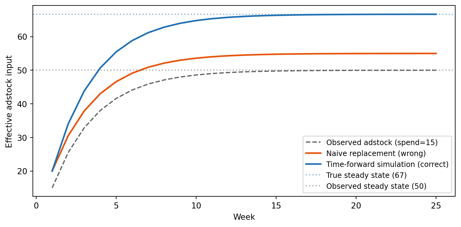
The naive approach (orange) produces adstock values close to the observed trajectory — the intervention barely shifts the effective input because the accumulated stock from the old spending history dominates. The correct approach (blue) re-builds the adstock accumulation from scratch using the counterfactual spend at every step, reaching the proper steady state.
This difference flows through the saturation function into sales, producing an underestimated causal effect if you skip time-forward simulation.
The fix: re-compute the temporal trajectory step by step
Time-forward simulation walks through each time step in order, computing the intervention’s effects and carrying them forward:
- Week 1: Set digital = 20. Compute adstock₁ = 20 (no prior state). Compute sales₁.
- Week 2: Set digital = 20. Compute adstock₂ = 20 + θ × adstock₁. Compute sales₂.
- Week 3: Set digital = 20. Compute adstock₃ = 20 + θ × adstock₂. Compute sales₃.
- …and so on until the trajectory converges to steady state.
Each step uses the simulated adstock from the previous step, not the observed one. This is what simulate_over="time" activates.
NoteThe same logic applies to lagged endogenous variables
If your model includes lag(sales) as a predictor of sales (an autoregressive term), the same cascade occurs: an intervention that changes sales at time t changes lag(sales) at time t+1, which changes sales at t+1, which changes lag(sales) at t+2, and so on. See the Panel Data Models example for a worked-through case with lagged promo effects.
Seeing it in pathmc
Here is a concrete model with adstock where we can compare the time-forward result to the time-averaged result. The key feature of the time-forward output is that it reveals the temporal shape of the effect — the ramp-up as adstock accumulates and the ramp-down as it decays.
n_weeks = 30
regions = ["North", "South"]
true_decay = 0.7
true_lam = 0.02
true_b = 30.0

rows = []
for region in regions:
    adstocked = 0.0
    for week in range(1, n_weeks + 1):
        x = rng.uniform(5, 25)
        adstocked = x + true_decay * adstocked
        sat = 1 - np.exp(-true_lam * adstocked)
        y = 50 + true_b * sat + rng.normal(scale=1.5)
        rows.append({"region": region, "week": week, "x": x, "y": y})

df = pd.DataFrame(rows)
model = pathmc.model(
"y ~ b*logistic_saturation(adstock(x, decay=theta), lam=lam)",
data=df,
panel={"unit": "region", "time": "week"},
pooling="partial",
)
model.fit(draws=500, tune=500, chains=2, random_seed=42, nuts_sampler="nutpie")/Users/benjamv/git/pathmc/pathmc/_model.py:165: UserWarning:
==============================================================================
PARTIAL POOLING WITH REDUNDANT INTERCEPT
==============================================================================
Your model uses pooling='partial' (random intercepts) but the following
equations include a formula intercept: 'y'.
This creates a NON-IDENTIFIABLE parameterization:
• beta[Intercept] (fixed global intercept)
• mu_alpha (mean of random intercepts)
Only their sum is identified by the data. This causes sampling divergences.
SOLUTION: Remove the intercept from your formula(s):
y ~ 0 + b*logistic_saturation(adstock(x, decay=theta), lam=lam)
The hierarchical mean mu_alpha will serve as the effective intercept.
==============================================================================
self._compile()
NUTS[nutpie]: [sigma_alpha_y, mu_alpha_y, alpha_y, lam, theta, beta_y, sigma_y]<xarray.DataTree>
Group: /
├── Group: /posterior
│ Dimensions: (chain: 2, draw: 500, unit: 2, y_predictors: 2,
│ mu_y_dim_0: 30, mu_y_dim_1: 2)
│ Coordinates:
│ * chain (chain) int64 16B 0 1
│ * draw (draw) int64 4kB 0 1 2 3 4 5 6 ... 494 495 496 497 498 499
│ * unit (unit) object 16B 'North' 'South'
│ * y_predictors (y_predictors) object 16B 'Intercept' 'x'
│ * mu_y_dim_0 (mu_y_dim_0) int64 240B 0 1 2 3 4 5 6 ... 24 25 26 27 28 29
│ * mu_y_dim_1 (mu_y_dim_1) int64 16B 0 1
│ Data variables:
│ mu_alpha_y (chain, draw) float64 8kB 8.956 11.8 16.99 ... 11.46 16.89
│ alpha_y (chain, draw, unit) float64 16kB 9.273 9.29 ... 17.32 16.84
│ beta_y (chain, draw, y_predictors) float64 16kB 37.82 ... 30.12
│ sigma_alpha_y (chain, draw) float64 8kB 0.3168 0.72 ... 0.6403 0.4401
│ lam (chain, draw) float64 8kB 0.04746 0.05095 ... 0.05396 0.05854
│ theta (chain, draw) float64 8kB 0.675 0.7 0.681 ... 0.6628 0.6525
│ sigma_y (chain, draw) float64 8kB 1.134 1.072 1.201 ... 1.103 1.281
│ mu_y (chain, draw, mu_y_dim_0, mu_y_dim_1) float64 480kB 59.27 ...
│ Attributes:
│ created_at: 2026-08-07T10:16:29.446124+00:00
│ creation_library: ArviZ
│ creation_library_version: 1.1.0
│ creation_library_language: Python
│ sample_dims: ['chain', 'draw']
│ inference_library: nutpie
│ inference_library_version: 0.16.10
│ sampling_time: 2.330571174621582
│ tuning_steps: 500
├── Group: /sample_stats
│ Dimensions: (chain: 2, draw: 500)
│ Coordinates:
│ * chain (chain) int64 16B 0 1
│ * draw (draw) int64 4kB 0 1 2 3 4 ... 495 496 497 498 499
│ Data variables: (12/20)
│ depth (chain, draw) uint64 8kB 6 6 7 4 6 5 ... 8 8 6 3 7
│ maxdepth_reached (chain, draw) bool 1kB False False ... False False
│ step_size (chain, draw) float64 8kB 0.1092 0.1287 ... 0.1027
│ transformation_update_id (chain, draw) int64 8kB 0 0 0 0 0 0 ... 0 0 0 0 0
│ step_size_bar (chain, draw) float64 8kB 0.1175 0.1175 ... 0.1089
│ mean_tree_accept (chain, draw) float64 8kB 0.8843 0.9971 ... 0.7995
│ ... ...
│ fisher_distance (chain, draw) float64 8kB 912.0 527.1 ... 129.3
│ transformation_index (chain, draw) int64 8kB 424 424 424 ... 424 424
│ diverging (chain, draw) bool 1kB False False ... False False
│ divergence_draw (chain, draw) uint64 8kB 0 0 0 0 0 0 ... 0 0 0 0 0
│ divergence_message (chain, draw) object 8kB nan nan nan ... nan nan
│ divergence_energy_error (chain, draw) float64 8kB nan nan nan ... nan nan
│ Attributes:
│ created_at: 2026-08-07T10:16:29.441327+00:00
│ creation_library: ArviZ
│ creation_library_version: 1.1.0
│ creation_library_language: Python
│ sample_dims: ['chain', 'draw']
│ inference_library: nutpie
│ inference_library_version: 0.16.10
│ inference_library_settings: {"sampler": "nuts", "adaptation": "diag", "s...
├── Group: /constant_data
│ Dimensions: (x_dim_0: 30, x_dim_1: 2)
│ Coordinates:
│ * x_dim_0 (x_dim_0) int64 240B 0 1 2 3 4 5 ... 24 25 26 27 28 29
│ * x_dim_1 (x_dim_1) int64 16B 0 1
│ Data variables:
│ _use_observed_carry int32 4B 1
│ x (x_dim_0, x_dim_1) float64 480B 20.48 16.3 ... 16.68
│ Attributes:
│ created_at: 2026-08-07T10:16:29.444433+00:00
│ creation_library: ArviZ
│ creation_library_version: 1.1.0
│ creation_library_language: Python
│ inference_library: pymc
│ inference_library_version: 6.0.1
│ sample_dims: []
├── Group: /observed_data
│ Dimensions: (y_dim_0: 30, y_dim_1: 2)
│ Coordinates:
│ * y_dim_0 (y_dim_0) int64 240B 0 1 2 3 4 5 6 7 8 ... 22 23 24 25 26 27 28 29
│ * y_dim_1 (y_dim_1) int64 16B 0 1
│ Data variables:
│ y (y_dim_0, y_dim_1) float64 480B 58.52 57.85 66.96 ... 70.41 68.38
│ Attributes:
│ created_at: 2026-08-07T10:16:29.445557+00:00
│ creation_library: ArviZ
│ creation_library_version: 1.1.0
│ creation_library_language: Python
│ inference_library: pymc
│ inference_library_version: 6.0.1
│ sample_dims: []
└── Group: /log_likelihood
Dimensions: (chain: 2, draw: 500, y_dim_0: 30, y_dim_1: 2)
Coordinates:
* chain (chain) int64 16B 0 1
* draw (draw) int64 4kB 0 1 2 3 4 5 6 7 ... 493 494 495 496 497 498 499
* y_dim_0 (y_dim_0) int64 240B 0 1 2 3 4 5 6 7 8 ... 22 23 24 25 26 27 28 29
* y_dim_1 (y_dim_1) int64 16B 0 1
Data variables:
y (chain, draw, y_dim_0, y_dim_1) float64 480kB -1.262 ... -1.174
Attributes:
created_at: 2026-08-07T10:16:29.546354+00:00
creation_library: ArviZ
creation_library_version: 1.1.0
creation_library_language: Python
inference_library: pymc
inference_library_version: 6.0.1
sample_dims: ['chain', 'draw']Now we intervene: boost x by 25% during weeks 8–18, then return to baseline. The time-forward simulation re-computes the adstock accumulation under the new spend pattern.
mean_x = df["x"].mean()
baseline_x = np.full(n_weeks, mean_x)
scenario_x = baseline_x.copy()
scenario_x[7:18] = mean_x * 1.25  # 25% boost, weeks 8-18

result_base = model.do(set={"x": baseline_x}, simulate_over="time")
result_scen = model.do(set={"x": scenario_x}, simulate_over="time")
contrast = result_scen - result_base
Code
weeks = np.arange(1, n_weeks + 1)
sales_by_time = contrast.by_time("y")

fig, ax = plt.subplots(figsize=(FIG_WIDTH, FIG_HEIGHT))
hdi_1 = az.hdi(sales_by_time.T, prob=0.94, axis=0)
ax.fill_between(weeks, hdi_1[:, 0], hdi_1[:, 1], alpha=0.15, color=COLOR_CORRECT)
ax.plot(
    weeks,
    sales_by_time.mean(axis=1),
    color=COLOR_CORRECT,
    lw=2,
    label="Incremental sales",
)
ax.axvspan(8, 18, alpha=0.08, color=COLOR_BOOST)
ax.axhline(0, color="black", ls=":", alpha=0.4)
ax.set_xlabel("Week")
ax.set_ylabel("Incremental sales (scenario − baseline)")
ax.legend()
plt.tight_layout()
plt.show()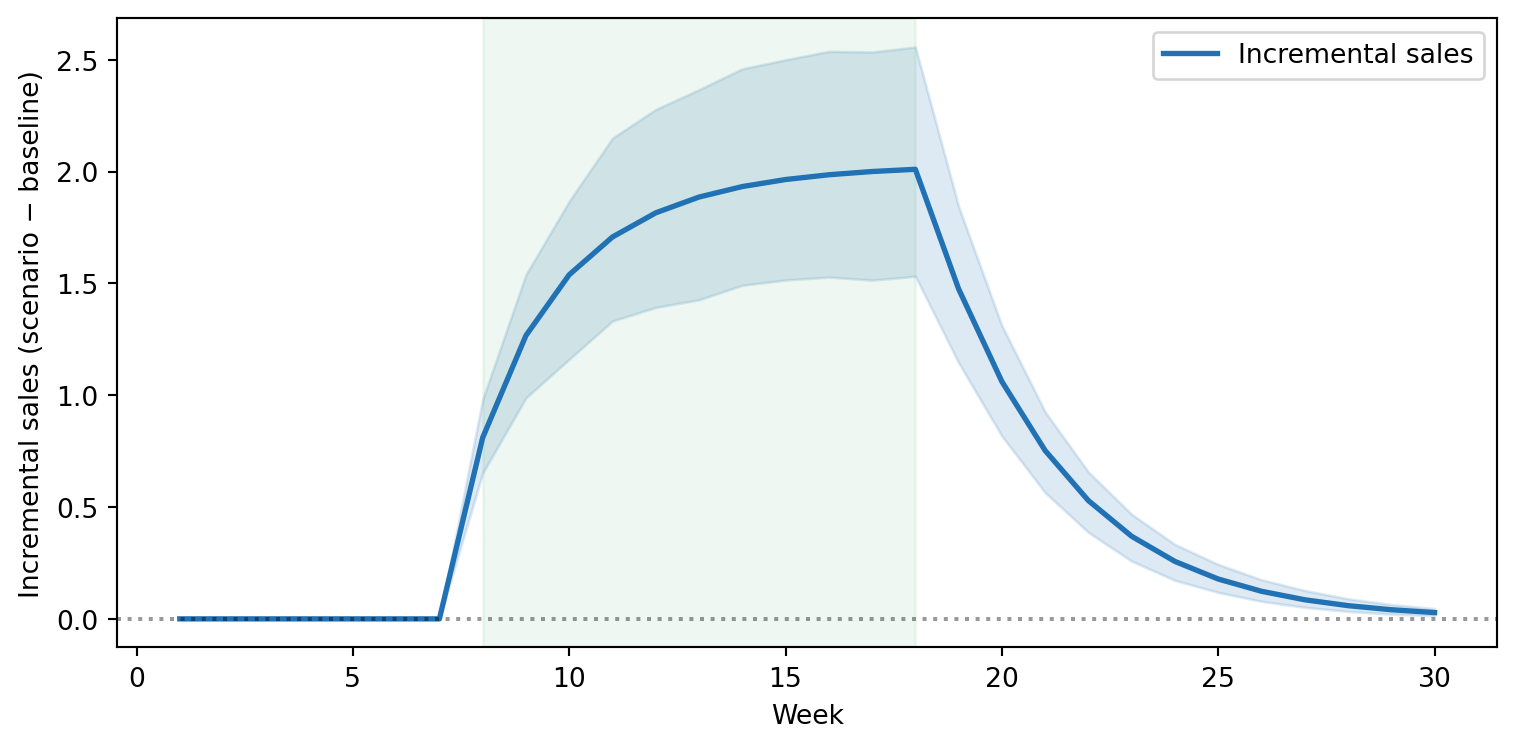
Three phases are visible:
- Before the boost (weeks 1–7): identical inputs, zero effect.
- During the boost (weeks 8–18): effect ramps up as the adstock stock accumulates from the extra spend.
- After the boost (weeks 19+): spend returns to baseline, but the accumulated adstock decays gradually — producing a tail of residual effect that a single-step intervention would miss entirely.
When do you need simulate_over="time"?
| Model feature | Creates temporal state? | Needs simulate_over="time"? |
|---|---|---|
| Random intercepts / slopes | No — unit-level shifts, no time dependency | No |
Trend term (week) |
No — deterministic, known at all time steps | No |
| Adstock transform | Yes — recursive accumulation across time | Yes |
Lagged exogenous (lag(promo)) |
Yes — previous value feeds current step | Yes |
Lagged endogenous (lag(sales)) |
Yes — previous outcome feeds current step | Yes |
The rule is simple: if any predictor at time t depends on a value computed at time t − 1, the intervention must walk through time in order.
TipIn practice
If your model has no adstock transforms and no lagged variables, you can use do() without simulate_over="time" — it works like a cross-sectional intervention applied independently at each (unit, time) point.
If your model has adstock or lagged variables, use do(simulate_over="time") so the temporal dynamics are re-computed under the intervention.
Summary
- Cross-sectional do() replaces a variable and forward-propagates in one step. This is correct when each observation is independent.
- Panel data does not automatically require time-forward simulation. Random intercepts, trend terms, and other non-temporal features don’t create dependencies between time steps.
- Adstock and lagged variables create temporal state. The adstock at time t depends on the adstock at t − 1. A lagged endogenous variable at t depends on the outcome at t − 1. Both create chains of dependency across time.
- Naive single-step replacement produces wrong counterfactuals because it uses the observed temporal state (from the pre-intervention history) instead of re-computing it under the intervention.
simulate_over="time"fixes this by walking through time in order, carrying simulated state forward from each step to the next.- The temporal shape matters. Time-forward simulation reveals ramp-up (stock accumulating) and ramp-down (stock decaying) dynamics that a single-step intervention collapses into a single number.
NoteReflection
Consider the temporal dynamics in your own models:
- Marketing / MMM: adstock transforms are the canonical example — ad spend accumulates and decays over weeks. A 15% budget increase this quarter doesn’t reach full effect until the stock builds up, and residual effects persist after the campaign ends.
- Public health: vaccination rates build herd immunity over time. A policy intervention that increases vaccination this month changes the susceptible population next month, affecting disease spread in a cascade that a single-step model misses.
- Finance: credit risk models often include lagged default rates or economic indicators. A policy shock to interest rates at time t alters default rates at t+1, which feeds back into portfolio risk at t+2.
If the effect you care about unfolds over time, your counterfactual simulation needs to unfold over time too.