Estimation Approaches

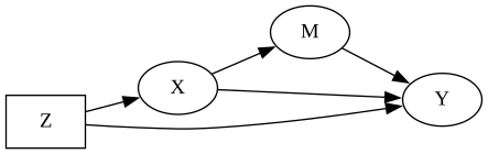
Structural models vs. regression adjustment: when to use which

Once you have a causal DAG, two estimation strategies target the same total effect of treatment on outcome. They agree on identification (which covariates block backdoor paths) and diverge on what you fit afterward. This page walks both paths on one graph so the shared first step is visible, not buried under different toy formulas.

The causal question and DAG

Suppose you want the total effect of X on Y when confounder Z opens a fork (Z → X and Z → Y), mediator M carries part of the effect (X → M → Y), and X also affects Y directly. The structural specification is:

X ~ Z
M ~ X
Y ~ M + X + Z

Build a data-free PathModel to inspect the graph before choosing an estimator.

import pathmc

spec = """
X ~ Z
M ~ X
Y ~ M + X + Z
"""

m = pathmc.model(spec)
m.graph()

Z is the only confounder on the fork. M lies on a causal path from X to Y and must not be treated as a covariate when estimating the total effect. The direct edge X → Y completes the system you will either fit in full or reduce for adjustment.

Shared identification

Both estimators start from the same DAG and the same backdoor logic. Before fitting anything, ask which variables must enter an adjustment set for the effect of X on Y.

m.adjustment_sets("X", "Y")

[{'Z'}]

Here the only backdoor path runs through Z, so the unique minimal adjustment set is {Z}. M is a mediator on the causal route from X to Y; conditioning on it would block part of the effect you want to measure.

The structural and regression-adjustment workflows differ after this step. One fits every equation and simulates interventions; the other fits a single outcome regression identified by {Z}.

The DAG is not optional for adjustment

A regression of Y on X and every column in your dataframe is not a causal estimator. Without the DAG you cannot know to adjust for Z rather than M, or that the empty set is valid on a different graph. adjustment_sets() and adjustment_model() exist so identification stays explicit.

Full structural model (structural g-computation)

On this DAG, specify all three equations and fit them jointly as one Bayesian model. The structural model is the causal model: each line is a mechanism, and uncertainty propagates through the system.

After fit(), intervene with do() or summarize a contrast with ate():

# | eval: false
m.fit(draws=1000, chains=2)
m.ate("Y", "X", values=(0.0, 1.0))
m.do(set={"X": 1.0})

do() applies graph surgery and structural g-computation: posterior draws are forwarded through the fitted equations for X, M, and Y. You do not hand-pick an adjustment set; the factorization encoded in the spec determines how an intervention on X propagates.

On this graph, path-specific queries are available because every mechanism is modeled, for example effect("X -> M -> Y") for the indirect route through M.

Strengths:

Answers any causal query from one fitted model: ATE, path-specific effects, probabilistic queries, counterfactual scenarios
Propagates uncertainty through the full DAG
Handles mediation, indirect effects, and multi-step chains without a separate adjustment argument
Supports do() on mediators (for example do(set={"M": 1.0})) when the question requires it

Weaknesses:

Requires correct specification of all equations, not only Y ~ …. Misspecifying M ~ X can bias downstream do() estimates even when the total effect of X on Y is the estimand
Computationally heavier when you only need one treatment-outcome contrast
Higher barrier to entry: you must defend the full system, not a single outcome equation

Regression adjustment (outcome-regression standardization)

Start from the same DAG and the same adjustment set {Z}. adjustment_model() reads the graph for identification, then builds a reduced outcome equation. It does not discard the DAG; it uses the DAG to decide what belongs in the regression.

A minimal data frame is enough to construct the adjustment facade (fitting is not shown here):

import pandas as pd

df = pd.DataFrame({"Z": [0.0], "X": [0.0], "M": [0.0], "Y": [0.0]})
adjusted = m.adjustment_model("X -> Y", data=df)
adjusted.adjustment_set

frozenset({'Z'})

adjusted.formula

'Y ~ X + Z'

The reduced formula is Y ~ X + Z: treatment plus the backdoor blockers, with no M in the covariate set. Outcome-regression standardization then:

Fits Y ~ X + Z (interactions and nonlinear terms are allowed on this equation)
Predicts Ŷ at X=1 and X=0 for each unit, holding Z at observed values
Averages the contrast to obtain ATE (and related estimands via cate(), att(), atu() after fit())

This is g-computation on one equation rather than on the full truncated factorization. For posterior draws and a numerical side-by-side with structural ate() on this same DAG, see SCM vs Regression Adjustment.

Bambi remains a useful external option when you need modeling features pathmc does not own: GAMs, rich crossed or nested multilevel formulas, and distributional regression beyond pathmc’s structural families. Bambi’s interpret module performs outcome-regression standardization on a hand-specified formula when identification assumptions hold.

Strengths:

For the total effect of X on Y, only the outcome equation and adjustment set need to be right; misspecifying M ~ X does not enter the adjustment likelihood
Computationally cheaper (one regression vs. a system of equations)
Handles nonlinearities, interactions, and non-Gaussian outcomes via standardization, not only a linear coefficient
Supports ATE, CATE, ATT, and ATU from one reduced model

Weaknesses:

Scoped to one treatment-outcome pair; a new query means a new adjustment model
Cannot decompose the effect through M (no effect("X -> M -> Y"))
Cannot intervene on M; only the designated treatment enters the standardization contrast
Does not encode the full generative story, only the total effect identified by the backdoor set

Assumptions vs. scope

These approaches are not in competition. They occupy different points on an assumptions-vs-scope trade-off curve.

	Structural model	Regression adjustment
DAG role	The DAG is the full generative model	The DAG identifies the adjustment set; one equation is fit
What you specify	All equations in the system	One outcome equation + adjustment set
What can go wrong	Misspecifying any equation biases do()	Only the outcome equation and adjustment set matter for the total effect
What you can query	Any variable, any intervention, any path	One treatment → one outcome
Estimands	ATE, CATE, ATT, ATU, path effects, P(Y \| do(X))	ATE, CATE, ATT, ATU
Computational cost	Fits N equations jointly	Fits 1 equation
pathmc entry point	`pathmc.model()` + do() / ate()	adjustment_model() + fit()

The single-regression approach with outcome-regression standardization is a fully capable estimator for the effect of one treatment on one outcome. It handles nonlinearities, interactions, and non-Gaussian outcomes; it produces ATE, CATE, ATT, and ATU with proper uncertainty. It is not a lesser tool. It is a more focused one.

The full structural model asks more of the analyst (specify all equations correctly) but rewards them with a richer object: path decomposition, multi-variable interventions, and the ability to query any variable under any combination of interventions.

When to use which

pathmc supports three estimation paths once you have a DAG and data. Pick based on the causal question and the modeling features you need.

Use a full structural model (pathmc.model() + do()) when:

You want to understand how an effect propagates through the system (direct vs. indirect effects, mediation)
You need to intervene on multiple variables or ask “what if” questions about different parts of the DAG
You want path-specific effects like effect("X → M → Y")
You want probabilistic queries like prob("Y > 0", set={"X": 1})
You are modeling a system where the mechanism matters, not just the total effect
You need panel do() with lags, adstock, or other structural transforms

Use native regression adjustment (adjustment_model()) when:

You have a clear treatment-outcome question and just need the total causal effect
You want pathmc to derive the adjustment set from the DAG and fit the reduced outcome equation in one workflow
You want to minimize modeling assumptions: specify one equation correctly rather than risk misspecifying the full system
Computational cost matters (large datasets, many posterior draws)
You want Bayesian uncertainty on ATE/CATE/ATT/ATU without leaving the pathmc API

Use external Bambi when:

You need GAMs, distributional models, or sophisticated crossed or nested random-effects structures pathmc does not provide
You already have a Bambi workflow and only need pathmc’s identification helpers upstream
You want Bambi’s interpret tooling on a formula you specify by hand

Use both together when:

You want pathmc’s identification helpers (adjustment_sets(), collider_warnings()) to determine what to adjust for, then estimate with adjustment_model() or hand off to Bambi for GAM or multilevel extensions

Where pathmc draws the line

pathmc is a DAG-aware Bayesian causal modeling package with two first-class estimators:

Structural modeling via pathmc.model(): specify the complete system of equations, fit jointly, and query via do() (structural g-computation).
Native regression adjustment via adjustment_model(): derive a backdoor adjustment set from the same DAG, fit a single outcome equation, and estimate via outcome-regression standardization.

Both estimators share the same identification layer: adjustment_sets(), is_identifiable(), and collider_warnings() work on the structural DAG regardless of which estimator you choose downstream.

For a worked side-by-side comparison of structural ate() and native adjustment_model().ate() on the confounder-mediator DAG above, see SCM vs Regression Adjustment.

pathmc does not try to replicate Bambi’s full regression modeling surface. When you need GAMs, rich multilevel formulas, or distributional regression beyond pathmc’s structural families, Bambi remains the right external tool. pathmc focuses on what it uniquely provides: joint structural equations with residual covariance, graph surgery via do(), panel time-forward simulation, transforms with estimable parameters, and DAG-native identification plus native backdoor adjustment.

For predictions(), comparisons(), and slopes() on both PathModel and AdjustmentModel, see Predictions, Comparisons, and Slopes and the interpret examples.