import numpy as np
import pandas as pd
import matplotlib.pyplot as plt
import arviz as az
import pymc as pm
import pathmc

FIG_WIDTH = 8
FIG_HEIGHT = 4

COLOR_TV = "#2171b5"
COLOR_DIGITAL = "#e6550d"
COLOR_BASELINE = "#636363"

COLOR_BRAND = "#2171b5"
COLOR_PERF = "#e6550d"
COLOR_SEARCH = "#31a354"
COLOR_INDIRECT = "#756bb1"Media Mix Models
Build MMMs of increasing complexity: adstock and saturation transforms, marketing funnel mediation, and hierarchical geo-varying effects.
A marketing analyst runs a regression of weekly sales on TV and digital spend. The model says TV is weak and digital is strong. Based on this, the team shifts budget from TV to digital — and six months later, sales are down. What went wrong?
Several things might have been missed:
- TV effects carry over across weeks and saturate at high spend levels — a linear regression captures neither
- TV spend also drove search traffic, which drove sales — the regression gave search credit for TV’s work
- TV was twice as effective in urban markets, but the model averaged over all regions
This notebook addresses all three problems with progressively richer models.
| Model | What it adds | Key pathmc features |
|---|---|---|
| 1. Transforms | Adstock carry-over + logistic saturation | adstock(), logistic_saturation(), panel mode |
| 2. Marketing funnel | Direct vs indirect effects through a mediator | Labeled coefficients, := defined parameters, effect() |
| 3. Hierarchical geo | Region-varying media coefficients | pooling={"slopes": [...]}, random slopes |
Each model adds a new dimension to the analysis. You can stop after any section and apply what you’ve learned.
Model 1: Adstock and saturation transforms
Two empirical regularities shape how advertising affects sales:
- Adstock: effects carry over across time periods — a TV ad this week still influences next week’s sales. Geometric carry-over: y_t = x_t + \text{decay} \cdot y_{t-1}.
- Logistic saturation: each additional unit of spend produces less incremental effect. y = 1 - \exp(-\lambda \cdot x).
This model captures both transforms in a panel of 4 regions over 30 weeks.
The causal structure
Simulate panel data
rng = np.random.default_rng(42)

regions = ["North", "South", "East", "West"]
n_weeks = 30
true_intercepts = {"North": 50, "South": 60, "East": 45, "West": 55}
true_decay_tv = 0.7
true_decay_dig = 0.5
true_lam_tv = 0.3
true_lam_dig = 0.4
true_b_tv = 8.0
true_b_dig = 6.0

rows = []
for region in regions:
    adstocked_tv = 0.0
    adstocked_dig = 0.0
    for week in range(1, n_weeks + 1):
        tv = rng.uniform(10, 50)
        digital = rng.uniform(5, 30)
        adstocked_tv = tv + true_decay_tv * adstocked_tv
        adstocked_dig = digital + true_decay_dig * adstocked_dig
        sat_tv = 1 - np.exp(-true_lam_tv * adstocked_tv)
        sat_dig = 1 - np.exp(-true_lam_dig * adstocked_dig)
        sales = (
            true_intercepts[region]
            + true_b_tv * sat_tv
            + true_b_dig * sat_dig
            + 0.1 * week
            + rng.normal(scale=1.5)
        )
        rows.append({
            "region": region,
            "week": week,
            "tv": tv,
            "digital": digital,
            "trend": week,
            "sales": sales,
        })

df = pd.DataFrame(rows)
print(f"Panel: {len(regions)} regions × {n_weeks} weeks = {len(df)} rows")
df.head()
Panel: 4 regions × 30 weeks = 120 rows| region | week | tv | digital | trend | sales | |
|---|---|---|---|---|---|---|
| 0 | North | 1 | 40.958242 | 15.971961 | 1 | 65.215558 |
| 1 | North | 2 | 37.894721 | 7.354434 | 2 | 62.233752 |
| 2 | North | 3 | 40.445588 | 24.651608 | 3 | 64.274784 |
| 3 | North | 4 | 28.015438 | 14.269951 | 4 | 65.566657 |
| 4 | North | 5 | 35.754605 | 25.569040 | 5 | 65.201264 |
Visualise sales by region
Code
REGION_COLORS = {
    "North": "#2171b5",
    "South": "#e6550d",
    "East": "#31a354",
    "West": "#756bb1",
}

fig, ax = plt.subplots(figsize=(FIG_WIDTH, FIG_HEIGHT))
for region in regions:
    d = df[df["region"] == region]
    ax.plot(d["week"], d["sales"], label=region, color=REGION_COLORS[region], alpha=0.8)
ax.set_xlabel("Week")
ax.set_ylabel("Sales")
ax.legend()
plt.tight_layout()
plt.show()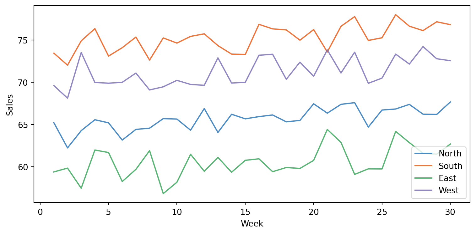
Specify and fit the model
The DSL supports transforms directly in the formula. Adstock and logistic saturation compose naturally: logistic_saturation(adstock(tv, decay=theta_tv), lam=lam_tv).
spec = """
sales ~ b_tv*logistic_saturation(adstock(tv, decay=theta_tv), lam=lam_tv)
      + b_dig*logistic_saturation(adstock(digital, decay=theta_dig), lam=lam_dig)
      + trend
"""

model = pathmc.model(
    spec,
    data=df,
    panel={"unit": "region", "time": "week"},
    pooling="partial",
)
model.graph()
/Users/juanitorduz/Documents/pathmc/pathmc/_model.py:192: UserWarning:
==============================================================================
PARTIAL POOLING WITH REDUNDANT INTERCEPT
==============================================================================
Your model uses pooling='partial' (random intercepts) but the following
equations include a formula intercept: 'sales'.
This creates a NON-IDENTIFIABLE parameterization:
• beta[Intercept] (fixed global intercept)
• mu_alpha (mean of random intercepts)
Only their sum is identified by the data. This causes sampling divergences.
SOLUTION: Remove the intercept from your formula(s):
sales ~ 0 + b_tv*logistic_saturation(adstock(tv, decay=theta_tv), lam=lam_tv) + b_dig*logistic_saturation(adstock(digital, decay=theta_dig), lam=lam_dig) + trend
The hierarchical mean mu_alpha will serve as the effective intercept.
==============================================================================
self._compile()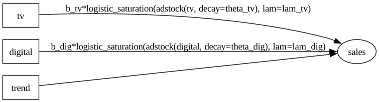
model.equations()\begin{aligned} \beta_{sales} &\sim \text{Normal}(mu=0,\, sigma=10) \\ \sigma_{sales} &\sim \text{HalfNormal}(sigma=1) \\ \mu_{alpha,sales} &\sim \text{Normal}(mu=0,\, sigma=10) \\ \sigma_{alpha,sales} &\sim \text{HalfNormal}(sigma=1) \\ \alpha_{sales} &\sim \text{Normal}(mu\_alpha,\, sigma\_alpha) \\ \theta_{tv} &\sim \text{Beta}(alpha=2,\, beta=2) \\ \lambda_{tv} &\sim \text{HalfNormal}(sigma=1) \\ \theta_{dig} &\sim \text{Beta}(alpha=2,\, beta=2) \\ \lambda_{dig} &\sim \text{HalfNormal}(sigma=1) \\[6pt] \mu_{sales} &= \beta_{0,\,sales} \\ &\quad + b_{tv} \cdot \operatorname{logistic\_saturation}(\operatorname{adstock}(\mathrm{tv},\, \theta_{tv}),\, \lambda_{tv}) \\ &\quad + b_{dig} \cdot \operatorname{logistic\_saturation}(\operatorname{adstock}(\mathrm{digital},\, \theta_{dig}),\, \lambda_{dig}) \\ &\quad + \mathrm{trend} \\ \mathrm{sales} &\sim \text{Normal}(\mu_{sales},\, \sigma_{sales}) \end{aligned}
pm.model_to_graphviz(model.pymc_model)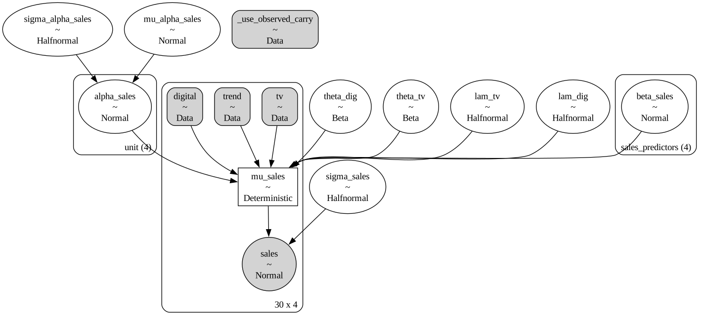
Sample
NoteSaturation–coefficient degeneracy
The b * saturation(lam * x) parameterization creates a funnel-shaped degeneracy between the coefficient and saturation steepness. This can cause divergences and max tree depth warnings. Consider tighter priors, reparameterization, or a non-centered saturation formulation if sampling is difficult.
model.fit(draws=500, tune=500, chains=4, random_seed=42, nuts_sampler="nutpie")NUTS[nutpie]: [sigma_alpha_sales, mu_alpha_sales, alpha_sales, lam_dig, theta_dig, lam_tv, theta_tv, beta_sales, sigma_sales]<xarray.DataTree>
Group: /
├── Group: /posterior
│ Dimensions: (chain: 4, draw: 500, unit: 4, sales_predictors: 4,
│ mu_sales_dim_0: 30, mu_sales_dim_1: 4)
│ Coordinates:
│ * chain (chain) int64 32B 0 1 2 3
│ * draw (draw) int64 4kB 0 1 2 3 4 5 ... 494 495 496 497 498 499
│ * unit (unit) object 32B 'East' 'North' 'South' 'West'
│ * sales_predictors (sales_predictors) object 32B 'Intercept' ... 'trend'
│ * mu_sales_dim_0 (mu_sales_dim_0) int64 240B 0 1 2 3 4 ... 25 26 27 28 29
│ * mu_sales_dim_1 (mu_sales_dim_1) int64 32B 0 1 2 3
│ Data variables:
│ mu_alpha_sales (chain, draw) float64 16kB 15.54 12.08 ... 14.11 10.6
│ alpha_sales (chain, draw, unit) float64 64kB 8.344 12.82 ... 12.95
│ beta_sales (chain, draw, sales_predictors) float64 64kB 18.91 ......
│ sigma_alpha_sales (chain, draw) float64 16kB 3.163 3.069 ... 4.389 4.092
│ lam_dig (chain, draw) float64 16kB 0.9388 0.4008 ... 1.677 1.244
│ theta_dig (chain, draw) float64 16kB 0.4657 0.6784 ... 0.478 0.259
│ lam_tv (chain, draw) float64 16kB 0.5893 1.093 ... 0.6076 0.7271
│ theta_tv (chain, draw) float64 16kB 0.5523 0.4182 ... 0.3037
│ sigma_sales (chain, draw) float64 16kB 1.444 1.242 ... 1.364 1.232
│ mu_sales (chain, draw, mu_sales_dim_0, mu_sales_dim_1) float64 2MB ...
│ Attributes:
│ created_at: 2026-08-06T09:00:00.188261+00:00
│ creation_library: ArviZ
│ creation_library_version: 1.1.0
│ creation_library_language: Python
│ sample_dims: ['chain', 'draw']
│ inference_library: nutpie
│ inference_library_version: 0.16.10
│ sampling_time: 9.702320098876953
│ tuning_steps: 500
├── Group: /sample_stats
│ Dimensions: (chain: 4, draw: 500)
│ Coordinates:
│ * chain (chain) int64 32B 0 1 2 3
│ * draw (draw) int64 4kB 0 1 2 3 4 ... 495 496 497 498 499
│ Data variables: (12/20)
│ depth (chain, draw) uint64 16kB 7 7 6 9 7 ... 8 8 7 6 7
│ maxdepth_reached (chain, draw) bool 2kB False False ... False False
│ step_size (chain, draw) float64 16kB 0.091 ... 0.07627
│ transformation_update_id (chain, draw) int64 16kB 0 0 0 0 0 0 ... 0 0 0 0 0
│ step_size_bar (chain, draw) float64 16kB 0.08424 ... 0.0818
│ mean_tree_accept (chain, draw) float64 16kB 0.9458 ... 0.8869
│ ... ...
│ fisher_distance (chain, draw) float64 16kB 192.3 875.2 ... 336.1
│ transformation_index (chain, draw) int64 16kB 423 423 423 ... 424 424
│ diverging (chain, draw) bool 2kB False False ... False False
│ divergence_draw (chain, draw) uint64 16kB 0 0 0 0 0 ... 0 0 0 0 0
│ divergence_message (chain, draw) object 16kB None None ... None None
│ divergence_energy_error (chain, draw) float64 16kB nan nan nan ... nan nan
│ Attributes:
│ created_at: 2026-08-06T09:00:00.182891+00:00
│ creation_library: ArviZ
│ creation_library_version: 1.1.0
│ creation_library_language: Python
│ sample_dims: ['chain', 'draw']
│ inference_library: nutpie
│ inference_library_version: 0.16.10
│ inference_library_settings: {"sampler": "nuts", "adaptation": "diag", "s...
├── Group: /constant_data
│ Dimensions: (tv_dim_0: 30, tv_dim_1: 4, trend_dim_0: 30,
│ trend_dim_1: 4, digital_dim_0: 30, digital_dim_1: 4)
│ Coordinates:
│ * tv_dim_0 (tv_dim_0) int64 240B 0 1 2 3 4 5 ... 24 25 26 27 28 29
│ * tv_dim_1 (tv_dim_1) int64 32B 0 1 2 3
│ * trend_dim_0 (trend_dim_0) int64 240B 0 1 2 3 4 5 ... 25 26 27 28 29
│ * trend_dim_1 (trend_dim_1) int64 32B 0 1 2 3
│ * digital_dim_0 (digital_dim_0) int64 240B 0 1 2 3 4 ... 25 26 27 28 29
│ * digital_dim_1 (digital_dim_1) int64 32B 0 1 2 3
│ Data variables:
│ _use_observed_carry int32 4B 1
│ tv (tv_dim_0, tv_dim_1) float64 960B 30.75 40.96 ... 14.68
│ trend (trend_dim_0, trend_dim_1) float64 960B 1.0 ... 30.0
│ digital (digital_dim_0, digital_dim_1) float64 960B 12.9 ......
│ Attributes:
│ created_at: 2026-08-06T09:00:00.185838+00:00
│ creation_library: ArviZ
│ creation_library_version: 1.1.0
│ creation_library_language: Python
│ inference_library: pymc
│ inference_library_version: 6.0.1
│ sample_dims: []
├── Group: /observed_data
│ Dimensions: (sales_dim_0: 30, sales_dim_1: 4)
│ Coordinates:
│ * sales_dim_0 (sales_dim_0) int64 240B 0 1 2 3 4 5 6 ... 23 24 25 26 27 28 29
│ * sales_dim_1 (sales_dim_1) int64 32B 0 1 2 3
│ Data variables:
│ sales (sales_dim_0, sales_dim_1) float64 960B 59.39 65.22 ... 72.55
│ Attributes:
│ created_at: 2026-08-06T09:00:00.187508+00:00
│ creation_library: ArviZ
│ creation_library_version: 1.1.0
│ creation_library_language: Python
│ inference_library: pymc
│ inference_library_version: 6.0.1
│ sample_dims: []
└── Group: /log_likelihood
Dimensions: (chain: 4, draw: 500, sales_dim_0: 30, sales_dim_1: 4)
Coordinates:
* chain (chain) int64 32B 0 1 2 3
* draw (draw) int64 4kB 0 1 2 3 4 5 6 ... 493 494 495 496 497 498 499
* sales_dim_0 (sales_dim_0) int64 240B 0 1 2 3 4 5 6 ... 23 24 25 26 27 28 29
* sales_dim_1 (sales_dim_1) int64 32B 0 1 2 3
Data variables:
sales (chain, draw, sales_dim_0, sales_dim_1) float64 2MB -1.287 ....
Attributes:
created_at: 2026-08-06T09:00:00.339593+00:00
creation_library: ArviZ
creation_library_version: 1.1.0
creation_library_language: Python
inference_library: pymc
inference_library_version: 6.0.1
sample_dims: ['chain', 'draw']Results
model.summary()| mean | sd | eti89_lb | eti89_ub | ess_bulk | ess_tail | r_hat | mcse_mean | mcse_sd | |
|---|---|---|---|---|---|---|---|---|---|
| mu_alpha_sales | 16.837746 | 8.499183 | 2.995657 | 30.952308 | 452.092545 | 488.882153 | 1.005460 | 0.400166 | 0.271679 |
| alpha_sales[East] | 9.781063 | 8.542131 | -4.052441 | 23.727070 | 440.272795 | 496.889444 | 1.007314 | 0.406408 | 0.274086 |
| alpha_sales[North] | 14.861014 | 8.549601 | 0.831881 | 28.655403 | 441.211507 | 513.276101 | 1.006976 | 0.406496 | 0.273621 |
| alpha_sales[South] | 24.371061 | 8.555258 | 10.368017 | 38.424566 | 443.114018 | 511.842263 | 1.007366 | 0.407149 | 0.274505 |
| alpha_sales[West] | 20.381788 | 8.548452 | 6.497423 | 34.426979 | 442.036478 | 507.291016 | 1.007563 | 0.406171 | 0.273502 |
| ... | ... | ... | ... | ... | ... | ... | ... | ... | ... |
| mu_sales[28, 3] | 72.661449 | 0.304190 | 72.161416 | 73.136943 | 1841.307626 | 1689.864978 | 0.999398 | 0.007064 | 0.005274 |
| mu_sales[29, 0] | 62.117398 | 0.341341 | 61.578622 | 62.647573 | 2087.139596 | 1724.232770 | 1.000244 | 0.007431 | 0.005950 |
| mu_sales[29, 1] | 67.243033 | 0.323034 | 66.730209 | 67.749988 | 2097.031074 | 1798.467705 | 1.001076 | 0.007091 | 0.005479 |
| mu_sales[29, 2] | 76.757288 | 0.315578 | 76.254383 | 77.253453 | 1940.932080 | 1713.139729 | 1.001262 | 0.007181 | 0.005043 |
| mu_sales[29, 3] | 72.764872 | 0.313873 | 72.246418 | 73.252226 | 1825.249232 | 1687.694213 | 0.999417 | 0.007312 | 0.005444 |
135 rows × 9 columns
model.effects_summary()| mean | sd | hdi_3% | hdi_97% | |
|---|---|---|---|---|
| name | ||||
| b_tv | 15.717122 | 8.314662 | -0.019059 | 31.517837 |
| b_dig | 16.422390 | 9.244993 | -1.642244 | 32.701125 |
The transform parameters should be close to the true values: theta_tv ≈ 0.7, theta_dig ≈ 0.5, lam_tv ≈ 0.3, lam_dig ≈ 0.4.
Posterior predictive check
The .predict() method runs posterior predictive sampling — a key diagnostic to verify that the model can reproduce the observed data patterns.
idata = model.predict()Sampling: [sales]Code
pp_var = "sales_obs" if "sales_obs" in idata.posterior_predictive else "sales"
pp = idata.posterior_predictive[pp_var]
pp_mean_2d = pp.mean(dim=("chain", "draw")).values
sorted_regions = sorted(regions)

fig, axes = plt.subplots(
    2, 2, figsize=(FIG_WIDTH, FIG_HEIGHT * 1.5), sharex=True, sharey=True
)
for ax, region in zip(axes.flat, regions):
    obs = df.loc[df["region"] == region, "sales"].values
    weeks = df.loc[df["region"] == region, "week"].values
    r_idx = sorted_regions.index(region)
    pp_region = pp_mean_2d[:, r_idx]

    ax.scatter(
        weeks,
        obs,
        s=20,
        alpha=0.6,
        color=REGION_COLORS[region],
        zorder=3,
        label="Observed",
    )
    ax.plot(
        weeks,
        pp_region,
        "-",
        alpha=0.8,
        color=REGION_COLORS[region],
        lw=2,
        zorder=4,
        label="Predicted mean",
    )
    ax.set_title(region, fontweight="bold")
    ax.legend(fontsize=7, loc="lower right")

fig.supxlabel("Week")
fig.supylabel("Sales")
plt.tight_layout()
plt.show()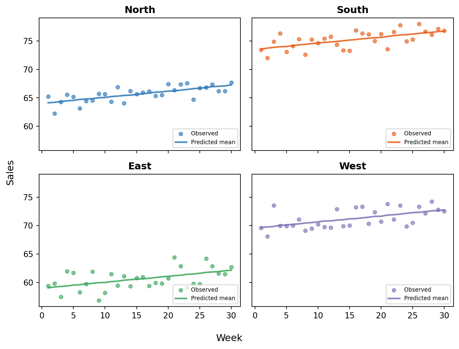
Counterfactual: what if we doubled TV spend?
Using time-forward do(), we simulate what sales would have been under a different spend scenario. The transforms (adstock + saturation) are automatically recomputed under the intervention.
r_baseline = model.do(
    set={"tv": 30.0, "digital": 15.0}, simulate_over="time", kind="mean"
)
r_double_tv = model.do(
    set={"tv": 60.0, "digital": 15.0}, simulate_over="time", kind="mean"
)
contrast = r_double_tv - r_baseline
/var/folders/cm/3dzy9rdd5s3672z0s1brjkvh0000gn/T/ipykernel_46076/2237643227.py:4: UserWarning: Intervention value 60.00 for 'tv' is outside the observed data range [10.71, 48.65]. Results are extrapolations and should be interpreted with caution.
r_double_tv = model.do(Code
fig, ax = plt.subplots(figsize=(FIG_WIDTH, FIG_HEIGHT * 1.2))

weeks = np.arange(1, n_weeks + 1)
avg_obs = df.groupby("week")["sales"].mean().values

pp_var = "sales_obs" if "sales_obs" in idata.posterior_predictive else "sales"
pp = idata.posterior_predictive[pp_var]
pp_mean_2d = pp.mean(dim=("chain", "draw")).values
pp_avg = pp_mean_2d.mean(axis=1) if pp_mean_2d.ndim == 2 else pp_mean_2d

ax.scatter(
    weeks,
    avg_obs,
    s=30,
    color="black",
    alpha=0.5,
    zorder=5,
    label="Observed (region avg)",
)
ax.plot(weeks, pp_avg, "-", color="black", lw=2, zorder=4, label="Model fit (PPC mean)")

bl_draws = r_baseline.draws("sales")
bl_mean = bl_draws.mean()
bl_hdi = r_baseline.hdi("sales", prob=0.94)
ax.axhspan(bl_hdi[0], bl_hdi[1], alpha=0.15, color=COLOR_BASELINE, zorder=1)
ax.axhline(
    bl_mean,
    color=COLOR_BASELINE,
    ls="--",
    lw=1.5,
    zorder=2,
    label=f"do(TV=30) = {bl_mean:.1f}",
)

dbl_draws = r_double_tv.draws("sales")
dbl_mean = dbl_draws.mean()
dbl_hdi = r_double_tv.hdi("sales", prob=0.94)
ax.axhspan(dbl_hdi[0], dbl_hdi[1], alpha=0.15, color=COLOR_TV, zorder=1)
ax.axhline(
    dbl_mean,
    color=COLOR_TV,
    ls="--",
    lw=1.5,
    zorder=2,
    label=f"do(TV=60) = {dbl_mean:.1f}",
)

mid_x = weeks[-1] + 1.5
ax.annotate(
    "",
    xy=(mid_x, dbl_mean),
    xytext=(mid_x, bl_mean),
    arrowprops=dict(arrowstyle="<->", color=COLOR_TV, lw=2),
)
lift = contrast.mean("sales")
ax.text(
    mid_x + 0.5,
    (bl_mean + dbl_mean) / 2,
    f"Δ = {lift:+.1f}",
    color=COLOR_TV,
    fontweight="bold",
    va="center",
    fontsize=10,
)

ax.set_xlabel("Week")
ax.set_ylabel("Sales (region average)")
ax.set_xlim(0, weeks[-1] + 4)
ax.legend(loc="lower right", fontsize=8)
plt.tight_layout()
plt.show()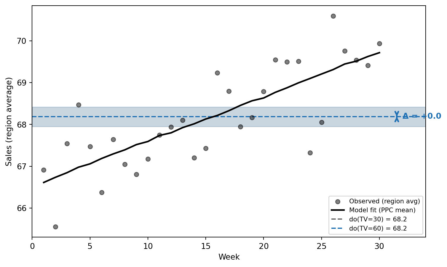
The horizontal bands show the do() operator’s predictions: what the model expects average sales to be under each fixed-spend scenario.
Code
fig, axes = plt.subplots(1, 2, figsize=(FIG_WIDTH, FIG_HEIGHT))

ax = axes[0]
for draws, color, label in [
    (r_baseline.draws("sales"), COLOR_BASELINE, "TV = 30 (baseline)"),
    (r_double_tv.draws("sales"), COLOR_TV, "TV = 60 (doubled)"),
]:
    x_kde, y_kde, _ = az.kde(draws)
    ax.plot(x_kde, y_kde, color=color, lw=2, label=label)
    ax.fill_between(x_kde, y_kde, alpha=0.3, color=color)
    ax.axvline(draws.mean(), color=color, ls="--", alpha=0.7, lw=1)
ax.set_xlabel("Mean sales")
ax.set_ylabel("Density")
ax.legend(fontsize=8)
ax.set_title("Scenario comparison")

ax = axes[1]
incr = contrast.draws("sales")
x_kde, y_kde, _ = az.kde(incr)
ax.plot(x_kde, y_kde, color=COLOR_TV, lw=2)
ax.fill_between(x_kde, y_kde, alpha=0.3, color=COLOR_TV)
hdi = contrast.hdi("sales", prob=0.94)
ax.axvspan(hdi[0], hdi[1], alpha=0.15, color=COLOR_TV, label="94% HDI")
ax.axvline(incr.mean(), color=COLOR_TV, ls="--", lw=1.5)
ax.axvline(0, color="black", ls=":", alpha=0.4)
ax.set_xlabel("Incremental sales (TV 60 − TV 30)")
ax.set_ylabel("Density")
ax.legend(fontsize=8)
ax.set_title("Causal effect of doubling TV")

plt.tight_layout()
plt.show()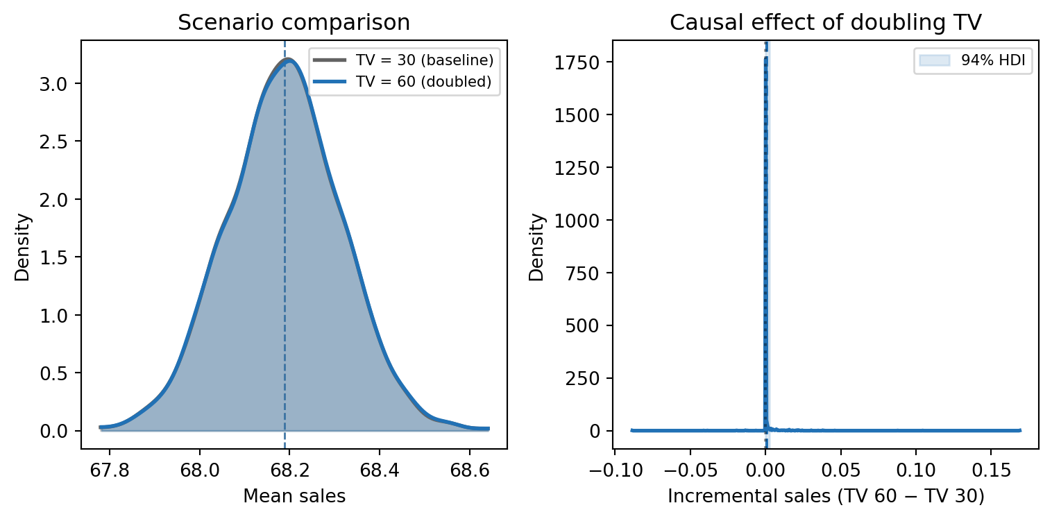
With saturation transforms, doubling TV spend does not double the effect — diminishing returns kick in.
Channel contribution
How much does each channel contribute to sales at the same spend level? We set each channel to 30 while holding the other at zero, then compare the lift over a no-spend baseline.
r_no_spend = model.do(
    set={"tv": 0.0, "digital": 0.0}, simulate_over="time", kind="mean"
)
r_tv_only = model.do(
    set={"tv": 30.0, "digital": 0.0}, simulate_over="time", kind="mean"
)
r_dig_only = model.do(
    set={"tv": 0.0, "digital": 30.0}, simulate_over="time", kind="mean"
)

tv_lift = r_tv_only - r_no_spend
dig_lift = r_dig_only - r_no_spend
/var/folders/cm/3dzy9rdd5s3672z0s1brjkvh0000gn/T/ipykernel_46076/1376975462.py:1: UserWarning: Intervention value 0.00 for 'tv' is outside the observed data range [10.71, 48.65]. Results are extrapolations and should be interpreted with caution.
r_no_spend = model.do(
/var/folders/cm/3dzy9rdd5s3672z0s1brjkvh0000gn/T/ipykernel_46076/1376975462.py:1: UserWarning: Intervention value 0.00 for 'digital' is outside the observed data range [5.18, 29.81]. Results are extrapolations and should be interpreted with caution.
r_no_spend = model.do(
/var/folders/cm/3dzy9rdd5s3672z0s1brjkvh0000gn/T/ipykernel_46076/1376975462.py:4: UserWarning: Intervention value 0.00 for 'digital' is outside the observed data range [5.18, 29.81]. Results are extrapolations and should be interpreted with caution.
r_tv_only = model.do(
/var/folders/cm/3dzy9rdd5s3672z0s1brjkvh0000gn/T/ipykernel_46076/1376975462.py:7: UserWarning: Intervention value 0.00 for 'tv' is outside the observed data range [10.71, 48.65]. Results are extrapolations and should be interpreted with caution.
r_dig_only = model.do(
/var/folders/cm/3dzy9rdd5s3672z0s1brjkvh0000gn/T/ipykernel_46076/1376975462.py:7: UserWarning: Intervention value 30.00 for 'digital' is outside the observed data range [5.18, 29.81]. Results are extrapolations and should be interpreted with caution.
r_dig_only = model.do(Code
fig, ax = plt.subplots(figsize=(FIG_WIDTH, FIG_HEIGHT))

for draws_obj, color, label in [
    (tv_lift, COLOR_TV, "TV (spend = 30)"),
    (dig_lift, COLOR_DIGITAL, "Digital (spend = 30)"),
]:
    draws = draws_obj.draws("sales")
    x_kde, y_kde, _ = az.kde(draws)
    ax.plot(x_kde, y_kde, color=color, lw=2, label=label)
    ax.fill_between(x_kde, y_kde, alpha=0.25, color=color)
    ax.axvline(draws.mean(), color=color, ls="--", alpha=0.7, lw=1)

ax.axvline(0, color="black", ls=":", alpha=0.4)
ax.set_xlabel("Incremental sales lift vs no spend")
ax.set_ylabel("Density")
ax.legend()
plt.tight_layout()
plt.show()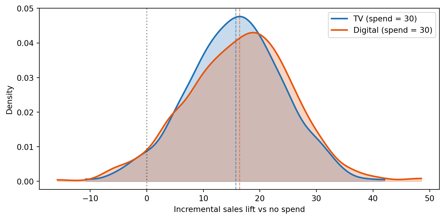
Diminishing returns curve
The saturation transform means each additional unit of spend produces less incremental sales. We trace out this curve by running do() at multiple spend levels.
Code
spend_levels = np.array([0, 5, 10, 20, 30, 40, 50, 60, 80])

tv_draws_list, dig_draws_list = [], []

for s in spend_levels:
    r_tv = model.do(
        set={"tv": float(s), "digital": 0.0}, simulate_over="time", kind="mean"
    )
    lift_tv = r_tv - r_no_spend
    tv_draws_list.append(lift_tv.draws("sales"))

    r_dig = model.do(
        set={"tv": 0.0, "digital": float(s)}, simulate_over="time", kind="mean"
    )
    lift_dig = r_dig - r_no_spend
    dig_draws_list.append(lift_dig.draws("sales"))

tv_draws_2d = np.column_stack(tv_draws_list)
dig_draws_2d = np.column_stack(dig_draws_list)

fig, ax = plt.subplots(figsize=(FIG_WIDTH, FIG_HEIGHT))
ax.plot(
    spend_levels, tv_draws_2d.mean(axis=0), "o-", color=COLOR_TV, label="TV", lw=2, ms=5
)
hdi_1 = az.hdi(tv_draws_2d, prob=0.94, axis=0)
ax.fill_between(spend_levels, hdi_1[:, 0], hdi_1[:, 1], alpha=0.15, color=COLOR_TV)
ax.plot(
    spend_levels,
    dig_draws_2d.mean(axis=0),
    "s-",
    color=COLOR_DIGITAL,
    label="Digital",
    lw=2,
    ms=5,
)
hdi_2 = az.hdi(dig_draws_2d, prob=0.94, axis=0)
ax.fill_between(spend_levels, hdi_2[:, 0], hdi_2[:, 1], alpha=0.15, color=COLOR_DIGITAL)
ax.set_xlabel("Channel spend (units)")
ax.set_ylabel("Incremental sales lift vs no spend")
ax.legend()
ax.axhline(0, color="black", ls=":", alpha=0.3)
plt.tight_layout()
plt.show()
/var/folders/cm/3dzy9rdd5s3672z0s1brjkvh0000gn/T/ipykernel_46076/1829389347.py:6: UserWarning: Intervention value 0.00 for 'tv' is outside the observed data range [10.71, 48.65]. Results are extrapolations and should be interpreted with caution.
r_tv = model.do(
/var/folders/cm/3dzy9rdd5s3672z0s1brjkvh0000gn/T/ipykernel_46076/1829389347.py:6: UserWarning: Intervention value 0.00 for 'digital' is outside the observed data range [5.18, 29.81]. Results are extrapolations and should be interpreted with caution.
r_tv = model.do(
/var/folders/cm/3dzy9rdd5s3672z0s1brjkvh0000gn/T/ipykernel_46076/1829389347.py:12: UserWarning: Intervention value 0.00 for 'tv' is outside the observed data range [10.71, 48.65]. Results are extrapolations and should be interpreted with caution.
r_dig = model.do(
/var/folders/cm/3dzy9rdd5s3672z0s1brjkvh0000gn/T/ipykernel_46076/1829389347.py:12: UserWarning: Intervention value 0.00 for 'digital' is outside the observed data range [5.18, 29.81]. Results are extrapolations and should be interpreted with caution.
r_dig = model.do(
/var/folders/cm/3dzy9rdd5s3672z0s1brjkvh0000gn/T/ipykernel_46076/1829389347.py:6: UserWarning: Intervention value 5.00 for 'tv' is outside the observed data range [10.71, 48.65]. Results are extrapolations and should be interpreted with caution.
r_tv = model.do(
/var/folders/cm/3dzy9rdd5s3672z0s1brjkvh0000gn/T/ipykernel_46076/1829389347.py:6: UserWarning: Intervention value 0.00 for 'digital' is outside the observed data range [5.18, 29.81]. Results are extrapolations and should be interpreted with caution.
r_tv = model.do(
/var/folders/cm/3dzy9rdd5s3672z0s1brjkvh0000gn/T/ipykernel_46076/1829389347.py:12: UserWarning: Intervention value 0.00 for 'tv' is outside the observed data range [10.71, 48.65]. Results are extrapolations and should be interpreted with caution.
r_dig = model.do(
/var/folders/cm/3dzy9rdd5s3672z0s1brjkvh0000gn/T/ipykernel_46076/1829389347.py:12: UserWarning: Intervention value 5.00 for 'digital' is outside the observed data range [5.18, 29.81]. Results are extrapolations and should be interpreted with caution.
r_dig = model.do(
/var/folders/cm/3dzy9rdd5s3672z0s1brjkvh0000gn/T/ipykernel_46076/1829389347.py:6: UserWarning: Intervention value 10.00 for 'tv' is outside the observed data range [10.71, 48.65]. Results are extrapolations and should be interpreted with caution.
r_tv = model.do(
/var/folders/cm/3dzy9rdd5s3672z0s1brjkvh0000gn/T/ipykernel_46076/1829389347.py:6: UserWarning: Intervention value 0.00 for 'digital' is outside the observed data range [5.18, 29.81]. Results are extrapolations and should be interpreted with caution.
r_tv = model.do(
/var/folders/cm/3dzy9rdd5s3672z0s1brjkvh0000gn/T/ipykernel_46076/1829389347.py:12: UserWarning: Intervention value 0.00 for 'tv' is outside the observed data range [10.71, 48.65]. Results are extrapolations and should be interpreted with caution.
r_dig = model.do(
/var/folders/cm/3dzy9rdd5s3672z0s1brjkvh0000gn/T/ipykernel_46076/1829389347.py:6: UserWarning: Intervention value 0.00 for 'digital' is outside the observed data range [5.18, 29.81]. Results are extrapolations and should be interpreted with caution.
r_tv = model.do(
/var/folders/cm/3dzy9rdd5s3672z0s1brjkvh0000gn/T/ipykernel_46076/1829389347.py:12: UserWarning: Intervention value 0.00 for 'tv' is outside the observed data range [10.71, 48.65]. Results are extrapolations and should be interpreted with caution.
r_dig = model.do(
/var/folders/cm/3dzy9rdd5s3672z0s1brjkvh0000gn/T/ipykernel_46076/1829389347.py:6: UserWarning: Intervention value 0.00 for 'digital' is outside the observed data range [5.18, 29.81]. Results are extrapolations and should be interpreted with caution.
r_tv = model.do(
/var/folders/cm/3dzy9rdd5s3672z0s1brjkvh0000gn/T/ipykernel_46076/1829389347.py:12: UserWarning: Intervention value 0.00 for 'tv' is outside the observed data range [10.71, 48.65]. Results are extrapolations and should be interpreted with caution.
r_dig = model.do(
/var/folders/cm/3dzy9rdd5s3672z0s1brjkvh0000gn/T/ipykernel_46076/1829389347.py:12: UserWarning: Intervention value 30.00 for 'digital' is outside the observed data range [5.18, 29.81]. Results are extrapolations and should be interpreted with caution.
r_dig = model.do(
/var/folders/cm/3dzy9rdd5s3672z0s1brjkvh0000gn/T/ipykernel_46076/1829389347.py:6: UserWarning: Intervention value 0.00 for 'digital' is outside the observed data range [5.18, 29.81]. Results are extrapolations and should be interpreted with caution.
r_tv = model.do(
/var/folders/cm/3dzy9rdd5s3672z0s1brjkvh0000gn/T/ipykernel_46076/1829389347.py:12: UserWarning: Intervention value 0.00 for 'tv' is outside the observed data range [10.71, 48.65]. Results are extrapolations and should be interpreted with caution.
r_dig = model.do(
/var/folders/cm/3dzy9rdd5s3672z0s1brjkvh0000gn/T/ipykernel_46076/1829389347.py:12: UserWarning: Intervention value 40.00 for 'digital' is outside the observed data range [5.18, 29.81]. Results are extrapolations and should be interpreted with caution.
r_dig = model.do(
/var/folders/cm/3dzy9rdd5s3672z0s1brjkvh0000gn/T/ipykernel_46076/1829389347.py:6: UserWarning: Intervention value 50.00 for 'tv' is outside the observed data range [10.71, 48.65]. Results are extrapolations and should be interpreted with caution.
r_tv = model.do(
/var/folders/cm/3dzy9rdd5s3672z0s1brjkvh0000gn/T/ipykernel_46076/1829389347.py:6: UserWarning: Intervention value 0.00 for 'digital' is outside the observed data range [5.18, 29.81]. Results are extrapolations and should be interpreted with caution.
r_tv = model.do(
/var/folders/cm/3dzy9rdd5s3672z0s1brjkvh0000gn/T/ipykernel_46076/1829389347.py:12: UserWarning: Intervention value 0.00 for 'tv' is outside the observed data range [10.71, 48.65]. Results are extrapolations and should be interpreted with caution.
r_dig = model.do(
/var/folders/cm/3dzy9rdd5s3672z0s1brjkvh0000gn/T/ipykernel_46076/1829389347.py:12: UserWarning: Intervention value 50.00 for 'digital' is outside the observed data range [5.18, 29.81]. Results are extrapolations and should be interpreted with caution.
r_dig = model.do(
/var/folders/cm/3dzy9rdd5s3672z0s1brjkvh0000gn/T/ipykernel_46076/1829389347.py:6: UserWarning: Intervention value 60.00 for 'tv' is outside the observed data range [10.71, 48.65]. Results are extrapolations and should be interpreted with caution.
r_tv = model.do(
/var/folders/cm/3dzy9rdd5s3672z0s1brjkvh0000gn/T/ipykernel_46076/1829389347.py:6: UserWarning: Intervention value 0.00 for 'digital' is outside the observed data range [5.18, 29.81]. Results are extrapolations and should be interpreted with caution.
r_tv = model.do(
/var/folders/cm/3dzy9rdd5s3672z0s1brjkvh0000gn/T/ipykernel_46076/1829389347.py:12: UserWarning: Intervention value 0.00 for 'tv' is outside the observed data range [10.71, 48.65]. Results are extrapolations and should be interpreted with caution.
r_dig = model.do(
/var/folders/cm/3dzy9rdd5s3672z0s1brjkvh0000gn/T/ipykernel_46076/1829389347.py:12: UserWarning: Intervention value 60.00 for 'digital' is outside the observed data range [5.18, 29.81]. Results are extrapolations and should be interpreted with caution.
r_dig = model.do(
/var/folders/cm/3dzy9rdd5s3672z0s1brjkvh0000gn/T/ipykernel_46076/1829389347.py:6: UserWarning: Intervention value 80.00 for 'tv' is outside the observed data range [10.71, 48.65]. Results are extrapolations and should be interpreted with caution.
r_tv = model.do(
/var/folders/cm/3dzy9rdd5s3672z0s1brjkvh0000gn/T/ipykernel_46076/1829389347.py:6: UserWarning: Intervention value 0.00 for 'digital' is outside the observed data range [5.18, 29.81]. Results are extrapolations and should be interpreted with caution.
r_tv = model.do(
/var/folders/cm/3dzy9rdd5s3672z0s1brjkvh0000gn/T/ipykernel_46076/1829389347.py:12: UserWarning: Intervention value 0.00 for 'tv' is outside the observed data range [10.71, 48.65]. Results are extrapolations and should be interpreted with caution.
r_dig = model.do(
/var/folders/cm/3dzy9rdd5s3672z0s1brjkvh0000gn/T/ipykernel_46076/1829389347.py:12: UserWarning: Intervention value 80.00 for 'digital' is outside the observed data range [5.18, 29.81]. Results are extrapolations and should be interpreted with caution.
r_dig = model.do(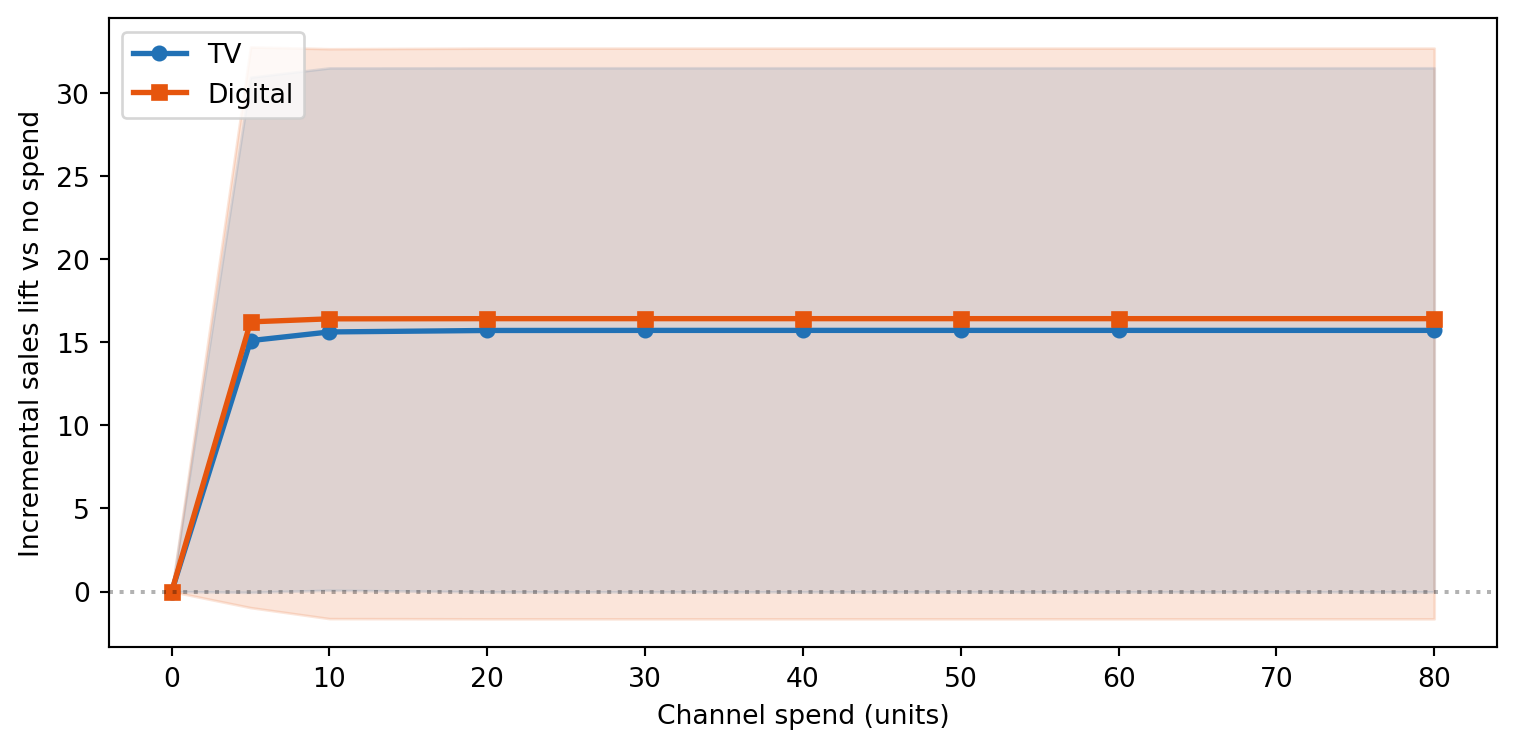
Model 1 captures the nonlinear response of each channel — adstock and saturation transform raw spend into effective exposure. But it treats each channel as an independent input. In reality, upper-funnel spend (brand campaigns, TV) doesn’t just drive sales directly — it also lifts search traffic, website visits, and other lower-funnel indicators that drive purchases in turn. Ignoring this funnel structure means upper-funnel spend looks weak while the downstream indicators it generated get all the credit.
Model 2: Marketing funnel with mediation
Upper-funnel advertising (brand campaigns, TV, YouTube) doesn’t just drive sales directly. It also lifts awareness, which surfaces as increased organic search traffic, website visits, and lower-funnel engagement — and those indicators drive purchases in turn.
This causal chain is a mediation structure: brand spend affects sales both directly and indirectly through a lower-funnel mediator. Standard MMMs that ignore this funnel face an attribution problem:
- Brand spend looks weak — part of its effect is “stolen” by search/organic variables
- Search traffic looks strong — it’s capturing brand’s indirect contribution
By modelling the funnel explicitly as a path model, we can decompose brand’s total effect into its direct and indirect components, and make better budget allocation decisions.
This model uses cross-sectional data to focus on the mediation structure itself — the funnel logic applies equally to panel and cross-sectional settings.
The causal structure
| Effect | Formula | Interpretation |
|---|---|---|
| Direct | c | Brand → Sales, not through search |
| Indirect | a × b | Brand → Search → Sales |
| Total | c + a × b | Full causal effect of brand spend |
Seasonality is a confounder of search traffic and sales — it must appear in both equations to avoid bias, but it is not on the causal path from brand spend to sales.
Simulate data
rng = np.random.default_rng(42)
n = 500

true_a = 0.6  # brand → search
true_b = 0.5  # search → sales
true_c = 0.25  # brand → sales (direct)
true_d = 0.7  # perf → sales
true_season_search = 0.4
true_season_sales = 0.3

season = rng.normal(size=n)
brand_spend = rng.uniform(0, 10, size=n)
perf_spend = rng.uniform(0, 8, size=n)

search_traffic = (
    true_a * brand_spend + true_season_search * season + rng.normal(scale=0.8, size=n)
)

sales = (
    true_c * brand_spend
    + true_b * search_traffic
    + true_d * perf_spend
    + true_season_sales * season
    + rng.normal(scale=1.0, size=n)
)

df = pd.DataFrame({
    "brand_spend": brand_spend,
    "perf_spend": perf_spend,
    "search_traffic": search_traffic,
    "season": season,
    "sales": sales,
})

true_indirect = true_a * true_b
true_total_brand = true_c + true_indirect

print(f"True direct brand effect:   {true_c}")
print(f"True indirect brand effect: {true_indirect}")
print(f"True total brand effect:    {true_total_brand}")
print(f"Fraction through funnel:    {true_indirect / true_total_brand:.0%}")
df.head()
True direct brand effect: 0.25
True indirect brand effect: 0.3
True total brand effect: 0.55
Fraction through funnel: 55%| brand_spend | perf_spend | search_traffic | season | sales | |
|---|---|---|---|---|---|
| 0 | 3.722616 | 5.996949 | 2.806107 | 0.304717 | 6.062537 |
| 1 | 1.536129 | 7.934462 | 0.597351 | -1.039984 | 5.955883 |
| 2 | 6.008404 | 4.251310 | 4.169178 | 0.750451 | 6.535680 |
| 3 | 1.196726 | 5.279966 | 1.716349 | 0.940565 | 4.349525 |
| 4 | 3.649194 | 2.419842 | 0.761513 | -1.951035 | 2.111758 |
Over half of brand’s total causal effect on sales flows through the search traffic mediator — invisible to a model that doesn’t represent the funnel.
Visualise the data
Code
fig, axes = plt.subplots(1, 3, figsize=(FIG_WIDTH, FIG_HEIGHT))

axes[0].scatter(brand_spend, search_traffic, alpha=0.3, s=10, color=COLOR_BRAND)
axes[0].set_xlabel("Brand spend")
axes[0].set_ylabel("Search traffic")

axes[1].scatter(search_traffic, sales, alpha=0.3, s=10, color=COLOR_SEARCH)
axes[1].set_xlabel("Search traffic")
axes[1].set_ylabel("Sales")

axes[2].scatter(brand_spend, sales, alpha=0.3, s=10, color=COLOR_BRAND)
axes[2].set_xlabel("Brand spend")
axes[2].set_ylabel("Sales")

plt.tight_layout()
plt.show()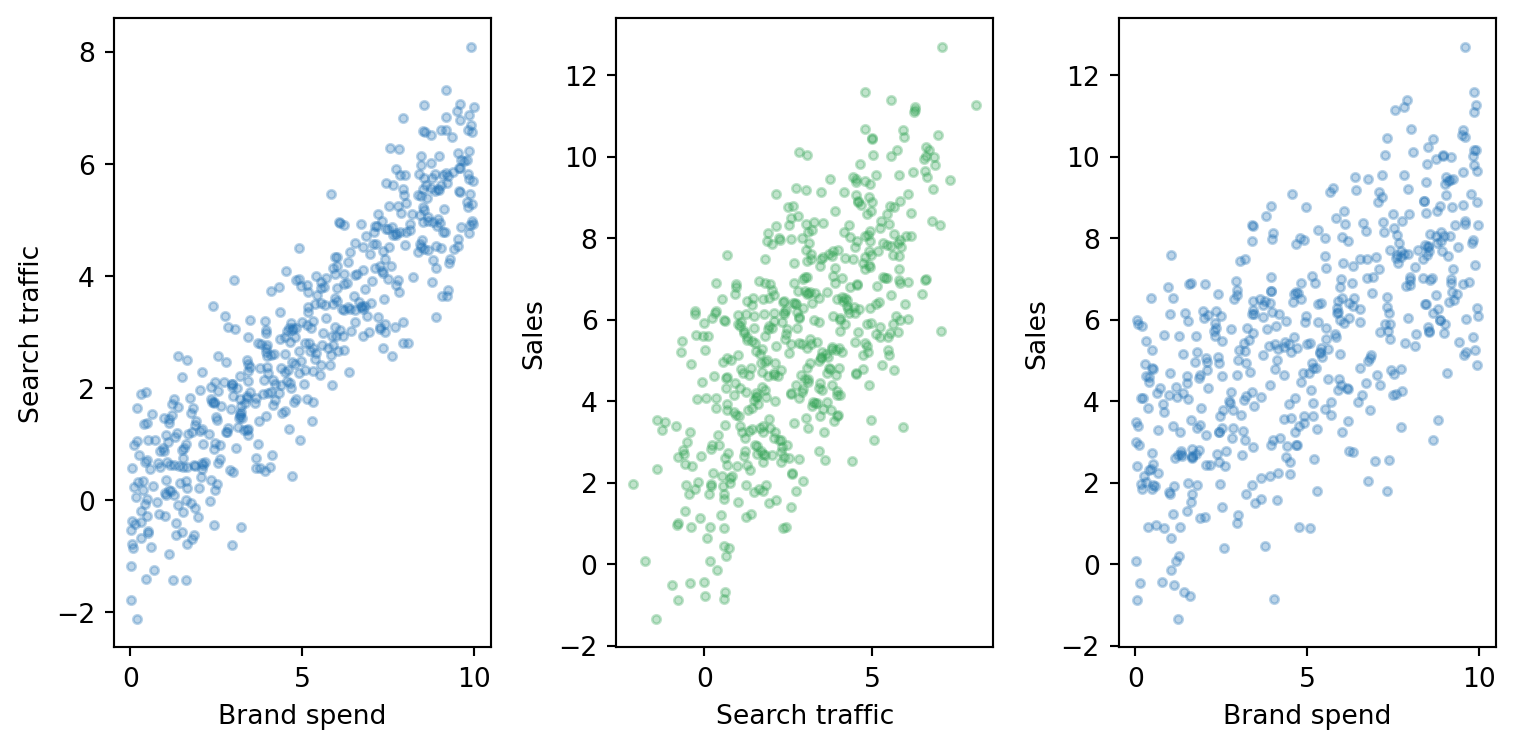
The attribution trap
WarningWhy naive regression misleads
Regressing sales ~ brand_spend + perf_spend + search_traffic + season estimates the direct effect of brand spend (≈ 0.25), not the total effect (≈ 0.55). By conditioning on the mediator search_traffic, the regression blocks the indirect path brand → search → sales.
This is correct if you want the direct effect. But for budget allocation — “how much total revenue does brand spend generate?” — you need the total effect, which requires modelling the funnel as a causal structure.
Specify and fit the path model
The spec encodes both equations in the funnel, with labeled coefficients for the paths we care about and a defined parameter for the indirect effect.
spec = """
search_traffic ~ a*brand_spend + season
sales ~ b*search_traffic + c*brand_spend + d*perf_spend + season
indirect := a*b
"""

model = pathmc.model(spec, data=df)
model.graph()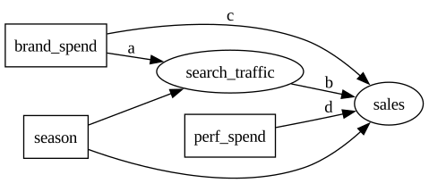
model.equations()\begin{aligned} \beta_{search,traffic} &\sim \text{Normal}(mu=0,\, sigma=10) \\ \sigma_{search,traffic} &\sim \text{HalfNormal}(sigma=1) \\ \beta_{sales} &\sim \text{Normal}(mu=0,\, sigma=10) \\ \sigma_{sales} &\sim \text{HalfNormal}(sigma=1) \\[6pt] \mu_{search,traffic} &= \beta_{0,\,search,traffic} + a \cdot \mathrm{brand\_spend} + \mathrm{season} \\ \mathrm{search\_traffic} &\sim \text{Normal}(\mu_{search,traffic},\, \sigma_{search,traffic}) \\ \mu_{sales} &= \beta_{0,\,sales} \\ &\quad + b \cdot \mathrm{search\_traffic} \\ &\quad + c \cdot \mathrm{brand\_spend} \\ &\quad + d \cdot \mathrm{perf\_spend} \\ &\quad + \mathrm{season} \\ \mathrm{sales} &\sim \text{Normal}(\mu_{sales},\, \sigma_{sales}) \\ indirect &\equiv a \cdot b \end{aligned}
pm.model_to_graphviz(model.pymc_model)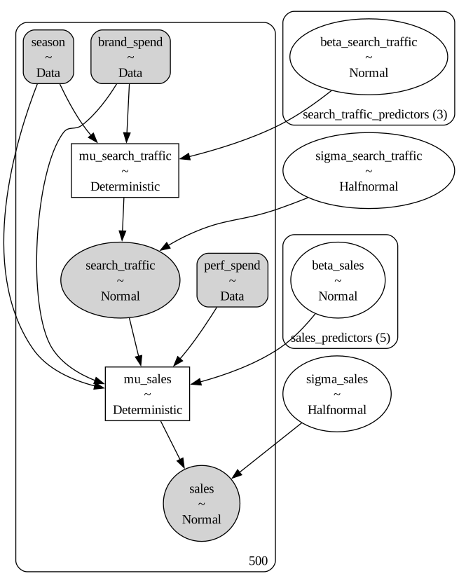
Sample
idata = model.fit(draws=1000, tune=1000, chains=4, random_seed=42)NUTS[nutpie]: [beta_sales, sigma_search_traffic, beta_search_traffic, sigma_sales]Results
model.summary()| mean | sd | eti89_lb | eti89_ub | ess_bulk | ess_tail | r_hat | mcse_mean | mcse_sd | |
|---|---|---|---|---|---|---|---|---|---|
| beta_sales[Intercept] | 0.081583 | 0.120139 | -0.110088 | 0.276364 | 1968.547416 | 2475.019511 | 1.001113 | 0.002710 | 0.001929 |
| beta_sales[search_traffic] | 0.478574 | 0.057069 | 0.388351 | 0.567732 | 1146.991858 | 1303.395394 | 1.000108 | 0.001692 | 0.001181 |
| beta_sales[brand_spend] | 0.265855 | 0.038683 | 0.204706 | 0.327044 | 1076.974423 | 1194.887719 | 0.999959 | 0.001184 | 0.000829 |
| beta_sales[perf_spend] | 0.673492 | 0.019396 | 0.642268 | 0.704704 | 2954.646998 | 2697.062940 | 1.001285 | 0.000357 | 0.000258 |
| beta_sales[season] | 0.266306 | 0.050911 | 0.184483 | 0.345914 | 3456.869293 | 3039.078581 | 1.000770 | 0.000865 | 0.000621 |
| ... | ... | ... | ... | ... | ... | ... | ... | ... | ... |
| mu_search_traffic[495] | 4.299073 | 0.054718 | 4.211255 | 4.387897 | 5655.774193 | 3610.591631 | 0.999821 | 0.000731 | 0.000520 |
| mu_search_traffic[496] | 4.359756 | 0.085859 | 4.220803 | 4.497655 | 4364.435489 | 3468.503487 | 1.000099 | 0.001298 | 0.000905 |
| mu_search_traffic[497] | -0.099343 | 0.067511 | -0.207252 | 0.006809 | 2479.310034 | 2514.399633 | 1.001426 | 0.001356 | 0.000997 |
| mu_search_traffic[498] | 1.849492 | 0.081341 | 1.721118 | 1.979515 | 4901.180413 | 3357.598340 | 1.000085 | 0.001163 | 0.000811 |
| mu_search_traffic[499] | 4.766490 | 0.079787 | 4.637414 | 4.893014 | 4004.564063 | 3637.932228 | 1.000353 | 0.001260 | 0.000880 |
1010 rows × 9 columns
model.effects_summary()| mean | sd | hdi_3% | hdi_97% | |
|---|---|---|---|---|
| name | ||||
| a | 0.619079 | 0.012134 | 0.595150 | 0.640697 |
| b | 0.478574 | 0.057069 | 0.373578 | 0.584829 |
| c | 0.265855 | 0.038683 | 0.191600 | 0.335555 |
| d | 0.673492 | 0.019396 | 0.636879 | 0.709670 |
| indirect | 0.296244 | 0.035551 | 0.234478 | 0.365996 |
TipReading the effects table
- a: brand → search (true = 0.6)
- b: search → sales (true = 0.5)
- c: brand → sales, direct (true = 0.25)
- d: perf → sales (true = 0.7)
- indirect: a × b (true = 0.3)
The total brand effect is c + indirect ≈ 0.55.
Path-specific effects
The effect() method multiplies posterior draws along a specified path, giving the full posterior distribution of path-specific effects.
indirect_effect = model.effect("brand_spend -> search_traffic -> sales")
print(f"Indirect effect (brand → search → sales): {indirect_effect}")

direct_effect = model.effect("brand_spend -> sales")
print(f"Direct effect (brand → sales):            {direct_effect}")
Indirect effect (brand → search → sales): EffectResult('brand_spend -> search_traffic -> sales', mean=0.2962, 94% HDI=[0.2345, 0.3660])
Direct effect (brand → sales): EffectResult('brand_spend -> sales', mean=0.2659, 94% HDI=[0.1916, 0.3356])Decomposing brand’s total effect
Code
fig, ax = plt.subplots(figsize=(FIG_WIDTH, FIG_HEIGHT))

a_draws = (
    idata
    .posterior["beta_search_traffic"]
    .sel(search_traffic_predictors="brand_spend")
    .values.flatten()
)
b_draws = (
    idata
    .posterior["beta_sales"]
    .sel(sales_predictors="search_traffic")
    .values.flatten()
)
c_draws = (
    idata.posterior["beta_sales"].sel(sales_predictors="brand_spend").values.flatten()
)
indirect_draws = a_draws * b_draws
total_draws = c_draws + indirect_draws

for draws, color, label, true_val in [
    (c_draws, COLOR_BRAND, "Direct (c)", true_c),
    (indirect_draws, COLOR_INDIRECT, "Indirect (a × b)", true_indirect),
    (total_draws, COLOR_SEARCH, "Total (c + a × b)", true_total_brand),
]:
    x_kde, y_kde, _ = az.kde(draws)
    ax.plot(x_kde, y_kde, color=color, lw=2, label=label)
    ax.fill_between(x_kde, y_kde, alpha=0.25, color=color)
    ax.axvline(true_val, color=color, ls="--", lw=1.5, alpha=0.7)

ax.axvline(0, color="black", ls=":", alpha=0.3)
ax.set_xlabel("Effect size (per unit brand spend)")
ax.set_ylabel("Density")
ax.legend()
plt.tight_layout()
plt.show()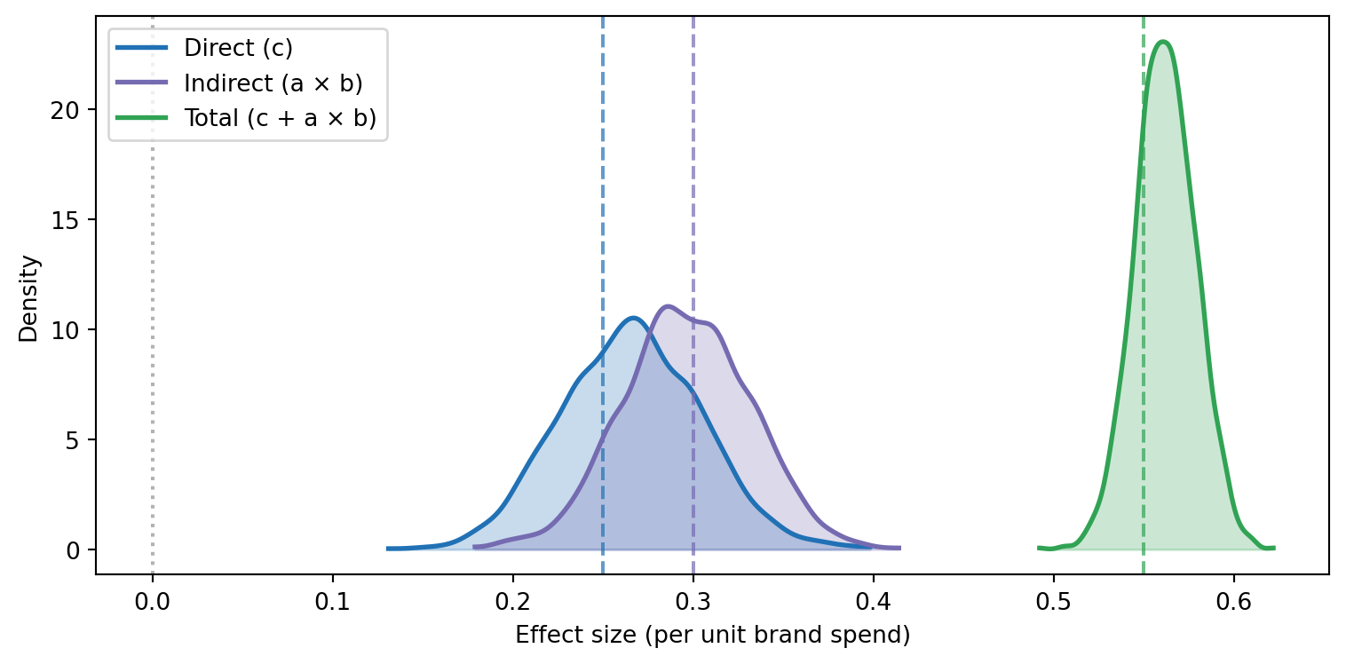
The indirect effect is comparable in magnitude to the direct effect — a naive regression that conditions on search traffic would miss roughly half of brand’s total contribution.
Identification and standardized effects
print(
    f"Is brand_spend → sales identifiable? {model.is_identifiable('brand_spend', 'sales')}"
)
print(
    f"Valid adjustment sets:                {model.adjustment_sets('brand_spend', 'sales')}"
)
Is brand_spend → sales identifiable? True
Valid adjustment sets: [set()]The empty set is a valid adjustment set because brand spend has no confounders (it is exogenous in this DAG).
model.standardized()| predictor | outcome | mean | sd | hdi_3% | hdi_97% | |
|---|---|---|---|---|---|---|
| name | ||||||
| a | brand_spend | search_traffic | 0.904832 | 0.017735 | 0.869859 | 0.936429 |
| b | search_traffic | sales | 0.376423 | 0.044888 | 0.293838 | 0.459998 |
| c | brand_spend | sales | 0.305628 | 0.044470 | 0.220264 | 0.385757 |
| d | perf_spend | sales | 0.611841 | 0.017621 | 0.578580 | 0.644707 |
Causal queries
Total causal effect of brand spend
The .ate() method computes the average treatment effect by contrasting two interventions — including both the direct path and the indirect path through search traffic:
brand_ate = model.ate("sales", "brand_spend", values=(2.0, 8.0))
brand_ate
ATE of brand_spend on sales
| Mean | 3.37 |
| 94% HDI | [3.19, 3.56] |
| P(> 0) | 1.00 |
| Draws | 4000 |
The ATE should be close to 0.55 × 6 = 3.3 — the total effect times the intervention size.
Probability query
p = model.prob("sales > 0", set={"brand_spend": 8.0})
print(f"P(sales > 0 | do(brand_spend=8)): {p:.2f}")
Sampling: [sales, search_traffic]P(sales > 0 | do(brand_spend=8)): 1.00Comparing channel effectiveness
Which channel produces more incremental sales per unit of spend?
r_base = model.do(set={"brand_spend": 0.0, "perf_spend": 0.0})

r_brand_only = model.do(set={"brand_spend": 5.0, "perf_spend": 0.0})
r_perf_only = model.do(set={"brand_spend": 0.0, "perf_spend": 5.0})

brand_lift = r_brand_only - r_base
perf_lift = r_perf_only - r_base
/var/folders/cm/3dzy9rdd5s3672z0s1brjkvh0000gn/T/ipykernel_46076/1173457870.py:1: UserWarning: Intervention value 0.00 for 'brand_spend' is outside the observed data range [0.01, 9.99]. Results are extrapolations and should be interpreted with caution.
r_base = model.do(set={"brand_spend": 0.0, "perf_spend": 0.0})
/var/folders/cm/3dzy9rdd5s3672z0s1brjkvh0000gn/T/ipykernel_46076/1173457870.py:1: UserWarning: Intervention value 0.00 for 'perf_spend' is outside the observed data range [0.00, 8.00]. Results are extrapolations and should be interpreted with caution.
r_base = model.do(set={"brand_spend": 0.0, "perf_spend": 0.0})
/var/folders/cm/3dzy9rdd5s3672z0s1brjkvh0000gn/T/ipykernel_46076/1173457870.py:3: UserWarning: Intervention value 0.00 for 'perf_spend' is outside the observed data range [0.00, 8.00]. Results are extrapolations and should be interpreted with caution.
r_brand_only = model.do(set={"brand_spend": 5.0, "perf_spend": 0.0})
/var/folders/cm/3dzy9rdd5s3672z0s1brjkvh0000gn/T/ipykernel_46076/1173457870.py:4: UserWarning: Intervention value 0.00 for 'brand_spend' is outside the observed data range [0.01, 9.99]. Results are extrapolations and should be interpreted with caution.
r_perf_only = model.do(set={"brand_spend": 0.0, "perf_spend": 5.0})Incremental sales from 5 units of brand spend:
brand_liftDoResult — 4000 draws, 5 variables
| variable | mean | 94% HDI |
|---|---|---|
| brand_spend | 5.00 | [5.00, 5.00] |
| season | 0.00 | [0.00, 0.00] |
| perf_spend | 0.00 | [0.00, 0.00] |
| search_traffic | 3.10 | [2.98, 3.20] |
| sales | 2.81 | [2.65, 2.97] |
Incremental sales from 5 units of performance spend:
perf_liftDoResult — 4000 draws, 5 variables
| variable | mean | 94% HDI |
|---|---|---|
| brand_spend | 0.00 | [0.00, 0.00] |
| season | 0.00 | [0.00, 0.00] |
| perf_spend | 5.00 | [5.00, 5.00] |
| search_traffic | 0.00 | [0.00, 0.00] |
| sales | 3.37 | [3.18, 3.55] |
Code
fig, ax = plt.subplots(figsize=(FIG_WIDTH, FIG_HEIGHT))

for lift_obj, color, label in [
    (brand_lift, COLOR_BRAND, "Brand (total, incl. funnel)"),
    (perf_lift, COLOR_PERF, "Performance (direct only)"),
]:
    draws = lift_obj.draws("sales")
    x_kde, y_kde, _ = az.kde(draws)
    ax.plot(x_kde, y_kde, color=color, lw=2, label=label)
    ax.fill_between(x_kde, y_kde, alpha=0.25, color=color)
    ax.axvline(draws.mean(), color=color, ls="--", alpha=0.7, lw=1)

ax.axvline(0, color="black", ls=":", alpha=0.3)
ax.set_xlabel("Incremental sales vs zero spend")
ax.set_ylabel("Density")
ax.legend()
plt.tight_layout()
plt.show()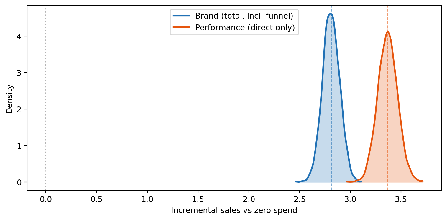
What does brand spend do to search traffic?
Because the model includes the funnel equation, do() also gives us the downstream effect on the mediator.
r_low = model.do(set={"brand_spend": 2.0})
r_high = model.do(set={"brand_spend": 8.0})r_lowDoResult — 4000 draws, 5 variables
| variable | mean | 94% HDI |
|---|---|---|
| brand_spend | 2.00 | [2.00, 2.00] |
| season | -0.01 | [-0.01, -0.01] |
| perf_spend | 4.04 | [4.04, 4.04] |
| search_traffic | 1.00 | [0.91, 1.10] |
| sales | 3.81 | [3.68, 3.93] |
r_highDoResult — 4000 draws, 5 variables
| variable | mean | 94% HDI |
|---|---|---|
| brand_spend | 8.00 | [8.00, 8.00] |
| season | -0.01 | [-0.01, -0.01] |
| perf_spend | 4.04 | [4.04, 4.04] |
| search_traffic | 4.72 | [4.62, 4.81] |
| sales | 7.18 | [7.05, 7.31] |
The expected lift in search traffic from 6 units of brand spend is true_a × 6.
Budget allocation
Code
spend_levels = np.array([0, 1, 2, 3, 5, 7, 10])

brand_draws_list, perf_draws_list = [], []

for s in spend_levels:
    r_b = model.do(set={"brand_spend": float(s), "perf_spend": 0.0})
    lift_b = r_b - r_base
    brand_draws_list.append(lift_b.draws("sales"))

    r_p = model.do(set={"brand_spend": 0.0, "perf_spend": float(s)})
    lift_p = r_p - r_base
    perf_draws_list.append(lift_p.draws("sales"))

brand_draws_2d = np.column_stack(brand_draws_list)
perf_draws_2d = np.column_stack(perf_draws_list)

fig, ax = plt.subplots(figsize=(FIG_WIDTH, FIG_HEIGHT))
ax.plot(
    spend_levels,
    brand_draws_2d.mean(axis=0),
    "o-",
    color=COLOR_BRAND,
    label="Brand (total)",
    lw=2,
    ms=5,
)
hdi_3 = az.hdi(brand_draws_2d, prob=0.94, axis=0)
ax.fill_between(spend_levels, hdi_3[:, 0], hdi_3[:, 1], alpha=0.15, color=COLOR_BRAND)
ax.plot(
    spend_levels,
    perf_draws_2d.mean(axis=0),
    "s-",
    color=COLOR_PERF,
    label="Performance",
    lw=2,
    ms=5,
)
hdi_4 = az.hdi(perf_draws_2d, prob=0.94, axis=0)
ax.fill_between(spend_levels, hdi_4[:, 0], hdi_4[:, 1], alpha=0.15, color=COLOR_PERF)

ax.plot(
    spend_levels,
    [true_total_brand * s for s in spend_levels],
    "--",
    color=COLOR_BRAND,
    alpha=0.5,
    label=f"True brand slope ({true_total_brand})",
)
ax.plot(
    spend_levels,
    [true_d * s for s in spend_levels],
    "--",
    color=COLOR_PERF,
    alpha=0.5,
    label=f"True perf slope ({true_d})",
)

ax.set_xlabel("Channel spend (units)")
ax.set_ylabel("Incremental sales vs zero spend")
ax.legend(fontsize=8)
ax.axhline(0, color="black", ls=":", alpha=0.3)
plt.tight_layout()
plt.show()
/var/folders/cm/3dzy9rdd5s3672z0s1brjkvh0000gn/T/ipykernel_46076/1959139574.py:6: UserWarning: Intervention value 0.00 for 'brand_spend' is outside the observed data range [0.01, 9.99]. Results are extrapolations and should be interpreted with caution.
r_b = model.do(set={"brand_spend": float(s), "perf_spend": 0.0})
/var/folders/cm/3dzy9rdd5s3672z0s1brjkvh0000gn/T/ipykernel_46076/1959139574.py:6: UserWarning: Intervention value 0.00 for 'perf_spend' is outside the observed data range [0.00, 8.00]. Results are extrapolations and should be interpreted with caution.
r_b = model.do(set={"brand_spend": float(s), "perf_spend": 0.0})
/var/folders/cm/3dzy9rdd5s3672z0s1brjkvh0000gn/T/ipykernel_46076/1959139574.py:10: UserWarning: Intervention value 0.00 for 'brand_spend' is outside the observed data range [0.01, 9.99]. Results are extrapolations and should be interpreted with caution.
r_p = model.do(set={"brand_spend": 0.0, "perf_spend": float(s)})
/var/folders/cm/3dzy9rdd5s3672z0s1brjkvh0000gn/T/ipykernel_46076/1959139574.py:10: UserWarning: Intervention value 0.00 for 'perf_spend' is outside the observed data range [0.00, 8.00]. Results are extrapolations and should be interpreted with caution.
r_p = model.do(set={"brand_spend": 0.0, "perf_spend": float(s)})
/var/folders/cm/3dzy9rdd5s3672z0s1brjkvh0000gn/T/ipykernel_46076/1959139574.py:6: UserWarning: Intervention value 0.00 for 'perf_spend' is outside the observed data range [0.00, 8.00]. Results are extrapolations and should be interpreted with caution.
r_b = model.do(set={"brand_spend": float(s), "perf_spend": 0.0})
/var/folders/cm/3dzy9rdd5s3672z0s1brjkvh0000gn/T/ipykernel_46076/1959139574.py:10: UserWarning: Intervention value 0.00 for 'brand_spend' is outside the observed data range [0.01, 9.99]. Results are extrapolations and should be interpreted with caution.
r_p = model.do(set={"brand_spend": 0.0, "perf_spend": float(s)})
/var/folders/cm/3dzy9rdd5s3672z0s1brjkvh0000gn/T/ipykernel_46076/1959139574.py:6: UserWarning: Intervention value 0.00 for 'perf_spend' is outside the observed data range [0.00, 8.00]. Results are extrapolations and should be interpreted with caution.
r_b = model.do(set={"brand_spend": float(s), "perf_spend": 0.0})
/var/folders/cm/3dzy9rdd5s3672z0s1brjkvh0000gn/T/ipykernel_46076/1959139574.py:10: UserWarning: Intervention value 0.00 for 'brand_spend' is outside the observed data range [0.01, 9.99]. Results are extrapolations and should be interpreted with caution.
r_p = model.do(set={"brand_spend": 0.0, "perf_spend": float(s)})
/var/folders/cm/3dzy9rdd5s3672z0s1brjkvh0000gn/T/ipykernel_46076/1959139574.py:6: UserWarning: Intervention value 0.00 for 'perf_spend' is outside the observed data range [0.00, 8.00]. Results are extrapolations and should be interpreted with caution.
r_b = model.do(set={"brand_spend": float(s), "perf_spend": 0.0})
/var/folders/cm/3dzy9rdd5s3672z0s1brjkvh0000gn/T/ipykernel_46076/1959139574.py:10: UserWarning: Intervention value 0.00 for 'brand_spend' is outside the observed data range [0.01, 9.99]. Results are extrapolations and should be interpreted with caution.
r_p = model.do(set={"brand_spend": 0.0, "perf_spend": float(s)})
/var/folders/cm/3dzy9rdd5s3672z0s1brjkvh0000gn/T/ipykernel_46076/1959139574.py:6: UserWarning: Intervention value 0.00 for 'perf_spend' is outside the observed data range [0.00, 8.00]. Results are extrapolations and should be interpreted with caution.
r_b = model.do(set={"brand_spend": float(s), "perf_spend": 0.0})
/var/folders/cm/3dzy9rdd5s3672z0s1brjkvh0000gn/T/ipykernel_46076/1959139574.py:10: UserWarning: Intervention value 0.00 for 'brand_spend' is outside the observed data range [0.01, 9.99]. Results are extrapolations and should be interpreted with caution.
r_p = model.do(set={"brand_spend": 0.0, "perf_spend": float(s)})
/var/folders/cm/3dzy9rdd5s3672z0s1brjkvh0000gn/T/ipykernel_46076/1959139574.py:6: UserWarning: Intervention value 0.00 for 'perf_spend' is outside the observed data range [0.00, 8.00]. Results are extrapolations and should be interpreted with caution.
r_b = model.do(set={"brand_spend": float(s), "perf_spend": 0.0})
/var/folders/cm/3dzy9rdd5s3672z0s1brjkvh0000gn/T/ipykernel_46076/1959139574.py:10: UserWarning: Intervention value 0.00 for 'brand_spend' is outside the observed data range [0.01, 9.99]. Results are extrapolations and should be interpreted with caution.
r_p = model.do(set={"brand_spend": 0.0, "perf_spend": float(s)})
/var/folders/cm/3dzy9rdd5s3672z0s1brjkvh0000gn/T/ipykernel_46076/1959139574.py:6: UserWarning: Intervention value 10.00 for 'brand_spend' is outside the observed data range [0.01, 9.99]. Results are extrapolations and should be interpreted with caution.
r_b = model.do(set={"brand_spend": float(s), "perf_spend": 0.0})
/var/folders/cm/3dzy9rdd5s3672z0s1brjkvh0000gn/T/ipykernel_46076/1959139574.py:6: UserWarning: Intervention value 0.00 for 'perf_spend' is outside the observed data range [0.00, 8.00]. Results are extrapolations and should be interpreted with caution.
r_b = model.do(set={"brand_spend": float(s), "perf_spend": 0.0})
/var/folders/cm/3dzy9rdd5s3672z0s1brjkvh0000gn/T/ipykernel_46076/1959139574.py:10: UserWarning: Intervention value 0.00 for 'brand_spend' is outside the observed data range [0.01, 9.99]. Results are extrapolations and should be interpreted with caution.
r_p = model.do(set={"brand_spend": 0.0, "perf_spend": float(s)})
/var/folders/cm/3dzy9rdd5s3672z0s1brjkvh0000gn/T/ipykernel_46076/1959139574.py:10: UserWarning: Intervention value 10.00 for 'perf_spend' is outside the observed data range [0.00, 8.00]. Results are extrapolations and should be interpreted with caution.
r_p = model.do(set={"brand_spend": 0.0, "perf_spend": float(s)})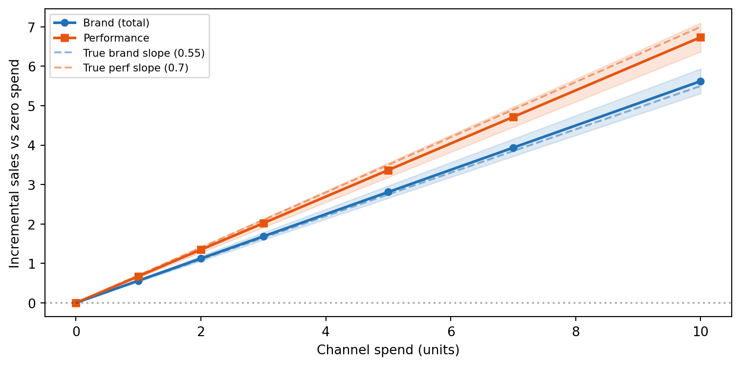
In this linear model the response curves are straight lines. Performance spend has a steeper marginal effect (0.7 vs 0.55 per unit), but brand spend is not far behind — and a flat regression that conditions on search traffic would underestimate brand at 0.25.
Model 2 separates direct from indirect effects, solving the attribution problem. But it treats all observations identically — a single coefficient for TV effectiveness everywhere. In practice, TV might drive more sales in one region due to higher viewership, while digital outperforms in another where the audience skews younger. A hierarchical model lets each region have its own media coefficients while borrowing strength from the full panel.
Model 3: Hierarchical geo-varying effects
Marketing channels rarely have the same effectiveness everywhere. This model fits a hierarchical panel MMM with geo-varying media coefficients using random slopes. Each region gets its own TV and digital effect, partially pooled toward a shared mean — borrowing strength across geos while allowing genuine heterogeneity.
No transforms (adstock, saturation) are used here; the focus is on the hierarchical structure itself. In practice, you would combine random slopes with the transforms from Model 1.
The model
For region g at week t:
\text{sales}_{g,t} = \alpha_g + (\beta_{\text{tv}} + u_{g,\text{tv}}) \cdot \text{tv}_{g,t} + (\beta_{\text{dig}} + u_{g,\text{dig}}) \cdot \text{digital}_{g,t} + \beta_{\text{trend}} \cdot t + \varepsilon_{g,t}
where \alpha_g is a random intercept and u_{g,\text{tv}}, u_{g,\text{dig}} are random slopes — each drawn from a shared normal with estimated mean and scale.
Simulate panel data
rng = np.random.default_rng(42)

regions = ["North", "South", "East", "West", "Central", "Coast"]
n_weeks = 40

true_mu_tv = 0.6
true_sigma_tv = 0.15
true_mu_dig = 0.4
true_sigma_dig = 0.10

true_tv_effects = {r: rng.normal(true_mu_tv, true_sigma_tv) for r in regions}
true_dig_effects = {r: rng.normal(true_mu_dig, true_sigma_dig) for r in regions}
true_intercepts = {r: rng.uniform(40, 70) for r in regions}

rows = []
for region in regions:
    for week in range(1, n_weeks + 1):
        tv = rng.uniform(5, 40)
        digital = rng.uniform(3, 25)
        sales = (
            true_intercepts[region]
            + true_tv_effects[region] * tv
            + true_dig_effects[region] * digital
            + 0.1 * week
            + rng.normal(scale=2.0)
        )
        rows.append({
            "region": region,
            "week": week,
            "tv": tv,
            "digital": digital,
            "trend": week,
            "sales": sales,
        })

df = pd.DataFrame(rows)
print(f"Panel: {len(regions)} regions × {n_weeks} weeks = {len(df)} rows")
df.head()
Panel: 6 regions × 40 weeks = 240 rows| region | week | tv | digital | trend | sales | |
|---|---|---|---|---|---|---|
| 0 | North | 1 | 33.967091 | 16.896617 | 1 | 87.953690 |
| 1 | North | 2 | 17.408409 | 24.355357 | 2 | 80.501138 |
| 2 | North | 3 | 32.243422 | 7.282052 | 3 | 84.506308 |
| 3 | North | 4 | 6.533132 | 6.394369 | 4 | 67.435582 |
| 4 | North | 5 | 31.066675 | 24.285214 | 5 | 88.876004 |
true_effects = pd.DataFrame({
    "region": regions,
    "tv_effect": [true_tv_effects[r] for r in regions],
    "digital_effect": [true_dig_effects[r] for r in regions],
})
true_effects| region | tv_effect | digital_effect | |
|---|---|---|---|
| 0 | North | 0.645708 | 0.412784 |
| 1 | South | 0.444002 | 0.368376 |
| 2 | East | 0.712568 | 0.398320 |
| 3 | West | 0.741085 | 0.314696 |
| 4 | Central | 0.307345 | 0.487940 |
| 5 | Coast | 0.404673 | 0.477779 |
Visualise sales by region
Code
fig, ax = plt.subplots(figsize=(FIG_WIDTH, FIG_HEIGHT))
palette = ["#2171b5", "#e6550d", "#31a354", "#756bb1", "#e7298a", "#636363"]
for region, color in zip(regions, palette):
    d = df[df["region"] == region]
    ax.plot(d["week"], d["sales"], label=region, color=color, alpha=0.7)
ax.set_xlabel("Week")
ax.set_ylabel("Sales")
ax.legend(ncol=3, fontsize=8)
plt.tight_layout()
plt.show()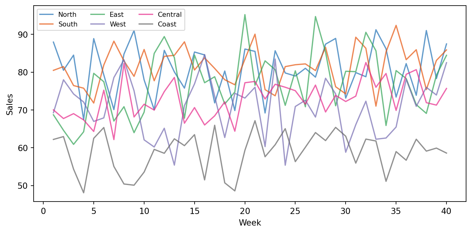
Specify and fit the model
The pooling argument controls the hierarchical structure:
"intercept": Truegives each region its own baseline sales level"slopes": ["tv", "digital"]gives each region its own media coefficients, partially pooled toward a shared mean
spec = """
sales ~ tv + digital + trend
"""

model = pathmc.model(
    spec,
    data=df,
    panel={"unit": "region", "time": "week"},
    pooling={"intercept": True, "slopes": ["tv", "digital"]},
)
/Users/juanitorduz/Documents/pathmc/pathmc/_model.py:192: UserWarning:
==============================================================================
PARTIAL POOLING WITH REDUNDANT INTERCEPT
==============================================================================
Your model uses pooling='partial' (random intercepts) but the following
equations include a formula intercept: 'sales'.
This creates a NON-IDENTIFIABLE parameterization:
• beta[Intercept] (fixed global intercept)
• mu_alpha (mean of random intercepts)
Only their sum is identified by the data. This causes sampling divergences.
SOLUTION: Remove the intercept from your formula(s):
sales ~ 0 + tv + digital + trend
The hierarchical mean mu_alpha will serve as the effective intercept.
==============================================================================
self._compile()model.equations()\begin{aligned} \beta_{sales} &\sim \text{Normal}(mu=0,\, sigma=10) \\ \sigma_{sales} &\sim \text{HalfNormal}(sigma=1) \\ \mu_{alpha,sales} &\sim \text{Normal}(mu=0,\, sigma=10) \\ \sigma_{alpha,sales} &\sim \text{HalfNormal}(sigma=1) \\ \alpha_{sales} &\sim \text{Normal}(mu\_alpha,\, sigma\_alpha) \\ \mu_{slope,sales,tv} &\sim \text{Normal}(mu=0,\, sigma=10) \\ \sigma_{slope,sales,tv} &\sim \text{HalfNormal}(sigma=1) \\ slope_{sales,tv} &\sim \text{Normal}(mu\_slope,\, sigma\_slope) \\ \mu_{slope,sales,digital} &\sim \text{Normal}(mu=0,\, sigma=10) \\ \sigma_{slope,sales,digital} &\sim \text{HalfNormal}(sigma=1) \\ slope_{sales,digital} &\sim \text{Normal}(mu\_slope,\, sigma\_slope) \\[6pt] \mu_{sales} &= \beta_{0,\,sales} \\ &\quad + \mathrm{tv} \\ &\quad + \mathrm{digital} \\ &\quad + \mathrm{trend} \\ \mathrm{sales} &\sim \text{Normal}(\mu_{sales},\, \sigma_{sales}) \end{aligned}
pm.model_to_graphviz(model.pymc_model)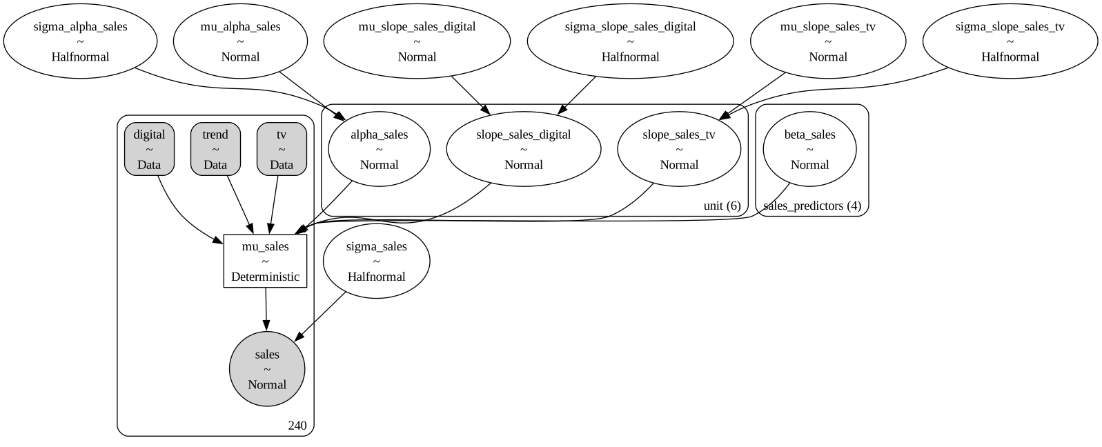
Sample
idata = model.fit(
    draws=1000, tune=1000, chains=4, random_seed=42, nuts_sampler="nutpie"
)
NUTS[nutpie]: [sigma_slope_sales_digital, mu_slope_sales_digital, slope_sales_digital, sigma_slope_sales_tv, mu_slope_sales_tv, slope_sales_tv, sigma_alpha_sales, mu_alpha_sales, alpha_sales, beta_sales, sigma_sales]Results
Population-level coefficients
The fixed effects represent the average media effectiveness across all regions.
model.summary()| mean | sd | eti89_lb | eti89_ub | ess_bulk | ess_tail | r_hat | mcse_mean | mcse_sd | |
|---|---|---|---|---|---|---|---|---|---|
| mu_slope_sales_digital | 0.116261 | 7.075341 | -12.300449 | 10.457807 | 39.399173 | 93.200835 | 1.097985 | 1.129427 | 0.734633 |
| slope_sales_digital[Central] | 0.247910 | 7.075323 | -12.181702 | 10.621338 | 39.414813 | 93.557943 | 1.097891 | 1.129358 | 0.734663 |
| slope_sales_digital[Coast] | 0.186634 | 7.075232 | -12.229308 | 10.500480 | 39.420791 | 93.311989 | 1.097962 | 1.129058 | 0.734280 |
| slope_sales_digital[East] | 0.040455 | 7.076071 | -12.416564 | 10.420734 | 39.367222 | 93.260209 | 1.097932 | 1.130285 | 0.734989 |
| slope_sales_digital[North] | 0.139388 | 7.076586 | -12.253488 | 10.494933 | 39.357667 | 93.906962 | 1.097963 | 1.129820 | 0.734810 |
| ... | ... | ... | ... | ... | ... | ... | ... | ... | ... |
| mu_sales[235] | 54.563342 | 0.526777 | 53.727405 | 55.407557 | 4379.152879 | 3625.032141 | 1.000623 | 0.007960 | 0.005592 |
| mu_sales[236] | 60.730525 | 0.517114 | 59.904777 | 61.558639 | 3998.153795 | 3473.385571 | 1.000731 | 0.008171 | 0.005939 |
| mu_sales[237] | 58.941573 | 0.376032 | 58.348282 | 59.568511 | 4182.626102 | 3279.723152 | 1.002907 | 0.005821 | 0.004018 |
| mu_sales[238] | 59.960705 | 0.621082 | 58.962847 | 60.963268 | 3632.357854 | 3219.771559 | 1.000129 | 0.010307 | 0.007239 |
| mu_sales[239] | 61.470610 | 0.379215 | 60.860804 | 62.079843 | 4010.356488 | 3065.703768 | 1.000639 | 0.005990 | 0.004205 |
269 rows × 9 columns
Geo-level TV effects
The random slopes capture how each region deviates from the population mean. The posterior for each region’s TV effect is the sum of the fixed effect and the region-specific deviation.
Code
fig, ax = plt.subplots(figsize=(FIG_WIDTH, FIG_HEIGHT * 1.2))

beta_tv = idata.posterior["beta_sales"].sel(sales_predictors="tv").values.flatten()
slope_tv = idata.posterior["slope_sales_tv"]

for i, region in enumerate(regions):
    region_slope = slope_tv.sel(unit=region).values.flatten()
    region_total = beta_tv + region_slope
    parts = ax.violinplot([region_total], positions=[i], showmedians=True, widths=0.7)
    for pc in parts["bodies"]:
        pc.set_facecolor(COLOR_TV)
        pc.set_alpha(0.4)
    for key in ["cmins", "cmaxes", "cbars", "cmedians"]:
        if key in parts:
            parts[key].set_color(COLOR_TV)

    ax.plot(i, true_tv_effects[region], "D", color="black", ms=6, zorder=5)

ax.set_xticks(range(len(regions)))
ax.set_xticklabels(regions)
ax.set_ylabel("TV effect on sales")
ax.axhline(
    true_mu_tv,
    color=COLOR_TV,
    ls="--",
    alpha=0.5,
    label=f"True pop. mean ({true_mu_tv})",
)
ax.legend(fontsize=8)
plt.tight_layout()
plt.show()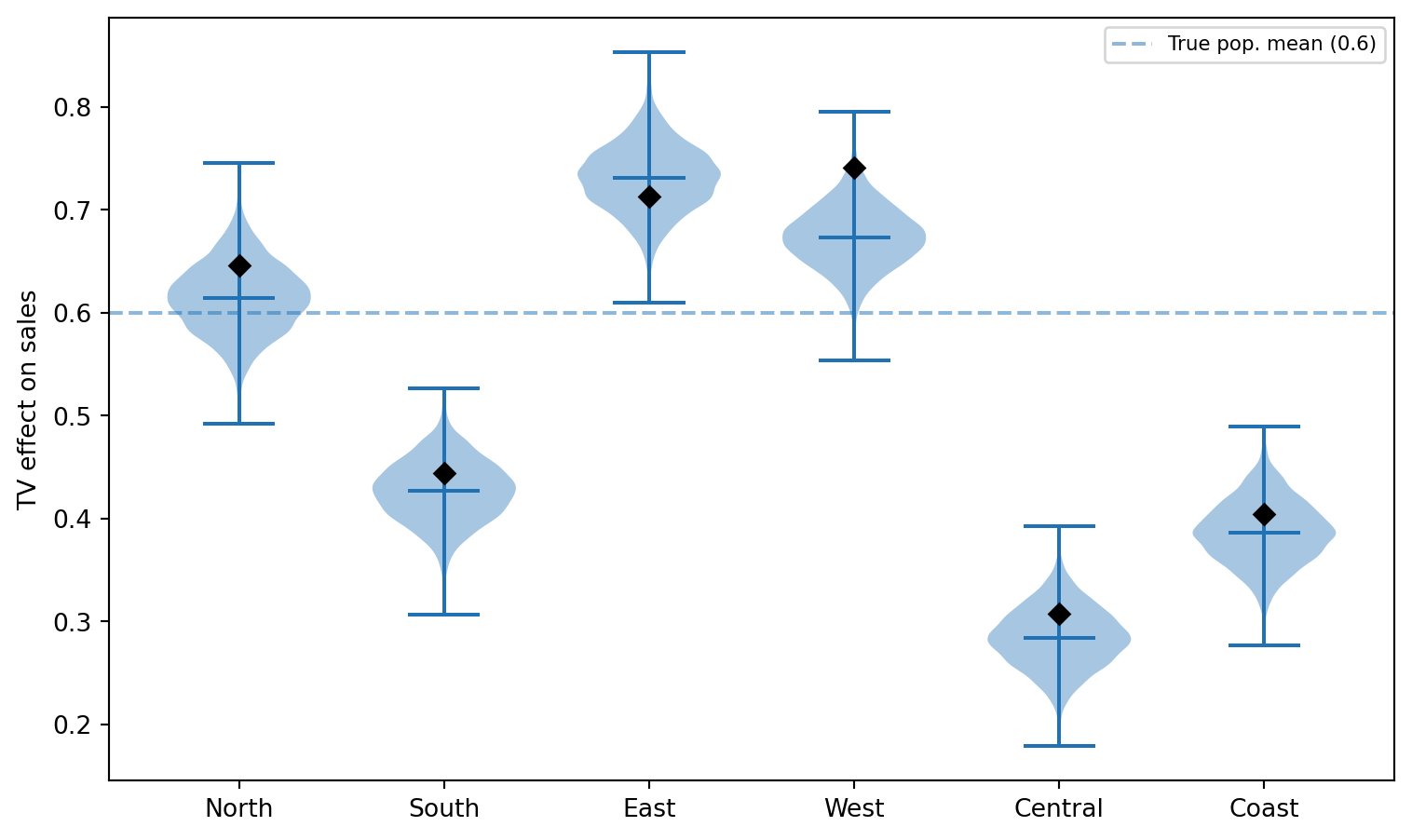
Black diamonds show the true geo-level effects used in the DGP.
Geo-level digital effects
Code
fig, ax = plt.subplots(figsize=(FIG_WIDTH, FIG_HEIGHT * 1.2))

beta_dig = (
    idata.posterior["beta_sales"].sel(sales_predictors="digital").values.flatten()
)
slope_dig = idata.posterior["slope_sales_digital"]

for i, region in enumerate(regions):
    region_slope = slope_dig.sel(unit=region).values.flatten()
    region_total = beta_dig + region_slope
    parts = ax.violinplot([region_total], positions=[i], showmedians=True, widths=0.7)
    for pc in parts["bodies"]:
        pc.set_facecolor(COLOR_DIGITAL)
        pc.set_alpha(0.4)
    for key in ["cmins", "cmaxes", "cbars", "cmedians"]:
        if key in parts:
            parts[key].set_color(COLOR_DIGITAL)

    ax.plot(i, true_dig_effects[region], "D", color="black", ms=6, zorder=5)

ax.set_xticks(range(len(regions)))
ax.set_xticklabels(regions)
ax.set_ylabel("Digital effect on sales")
ax.axhline(
    true_mu_dig,
    color=COLOR_DIGITAL,
    ls="--",
    alpha=0.5,
    label=f"True pop. mean ({true_mu_dig})",
)
ax.legend(fontsize=8)
plt.tight_layout()
plt.show()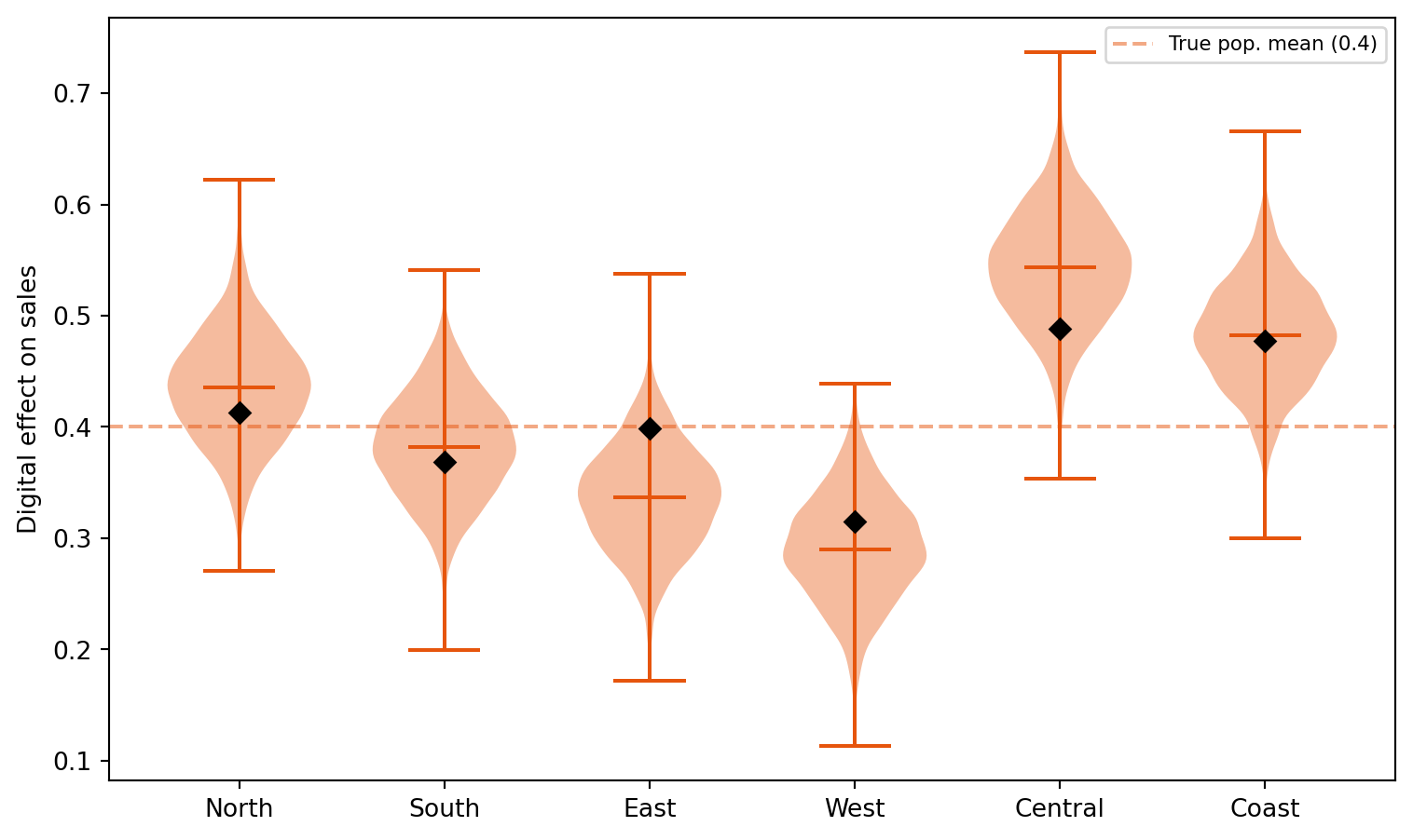
Shrinkage
Partial pooling pulls extreme geo estimates toward the group mean. Regions with less data or noisier observations are shrunk more — the model borrows strength from the full panel.
Code
fig, ax = plt.subplots(figsize=(FIG_WIDTH, FIG_HEIGHT))

for channel, beta_draws, slope_var, true_effects_dict, color, label in [
    ("tv", beta_tv, slope_tv, true_tv_effects, COLOR_TV, "TV"),
    ("digital", beta_dig, slope_dig, true_dig_effects, COLOR_DIGITAL, "Digital"),
]:
    true_vals = []
    post_means = []
    for region in regions:
        region_slope = slope_var.sel(unit=region).values.flatten()
        region_total = beta_draws + region_slope
        true_vals.append(true_effects_dict[region])
        post_means.append(region_total.mean())

    ax.scatter(true_vals, post_means, color=color, s=50, label=label, zorder=3)
    pop_mean = beta_draws.mean()
    ax.axhline(pop_mean, color=color, ls="--", alpha=0.3)

lims = ax.get_xlim()
ax.plot(lims, lims, "k:", alpha=0.3, label="Perfect recovery")
ax.set_xlabel("True geo-level effect")
ax.set_ylabel("Posterior mean")
ax.legend(fontsize=8)
plt.tight_layout()
plt.show()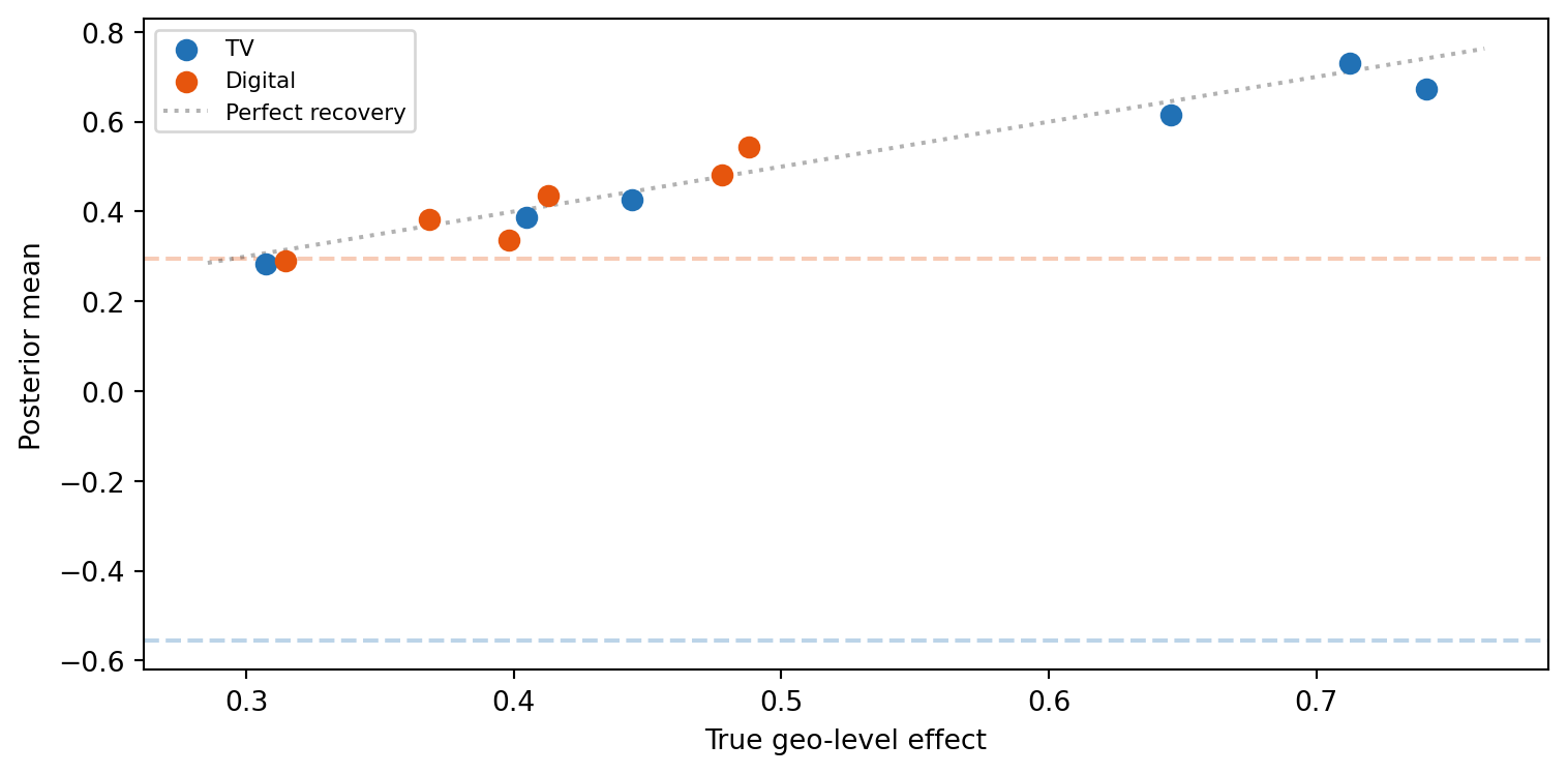
Hierarchical scale recovery
The estimated between-geo standard deviation tells us how much heterogeneity the model detected.
sigma_tv_post = idata.posterior["sigma_slope_sales_tv"].values.flatten()
sigma_dig_post = idata.posterior["sigma_slope_sales_digital"].values.flatten()

print(
    f"sigma_tv:  posterior mean = {sigma_tv_post.mean():.3f}  (true = {true_sigma_tv})"
)
print(
    f"sigma_dig: posterior mean = {sigma_dig_post.mean():.3f}  (true = {true_sigma_dig})"
)
sigma_tv: posterior mean = 0.248 (true = 0.15)
sigma_dig: posterior mean = 0.142 (true = 0.1)Causal queries with geo-varying effects
The do() operator propagates both random intercepts and random slopes, so interventional queries reflect the full heterogeneity across geos.
Average treatment effect
.ate() computes the population-average causal effect by contrasting two intervention levels:
ate_tv = model.ate("sales", "tv", values=(10.0, 30.0))
ate_tv
ATE of tv on sales
| Mean | 10.39 |
| 94% HDI | [9.92, 10.90] |
| P(> 0) | 1.00 |
| Draws | 4000 |
The expected population-average effect is 0.6 × 20 = 12.0.
Comparing channels
ate_dig = model.ate("sales", "digital", values=(5.0, 20.0))
ate_dig
ATE of digital on sales
| Mean | 6.18 |
| 94% HDI | [5.59, 6.78] |
| P(> 0) | 1.00 |
| Draws | 4000 |
The expected effect for digital is 0.4 × 15 = 6.0.
Probability query
p = model.prob("sales > 10", set={"tv": 30.0}, kind="predictive")
print(f"P(sales > 10 | do(tv=30)): {p:.2f}")
Sampling: [sales]P(sales > 10 | do(tv=30)): 1.00Summary
- Adstock and saturation transforms capture the nonlinear response of advertising channels — carry-over across time periods and diminishing returns at high spend levels.
- Posterior predictive checks verify that the model can reproduce observed data patterns before running causal queries.
- do() queries with transforms automatically recompute the full transform pipeline under the intervention, capturing how effects change nonlinearly with spend.
- The marketing funnel is a mediation structure. Upper-funnel spend drives sales both directly and through lower-funnel indicators like search traffic. Conditioning on the mediator blocks the indirect path and underestimates upper-funnel’s contribution.
- Path analysis with labeled coefficients gives the full posterior of direct, indirect, and total effects — the quantities that matter for budget allocation.
- Hierarchical panel models let each region have its own media coefficient while borrowing strength from the full panel through partial pooling.
- Random slopes reveal genuine heterogeneity in channel effectiveness across geographies, enabling region-specific budget allocation.
NoteReflection
In your own marketing data:
- Which channels might have indirect effects through downstream indicators like search traffic, app installs, or social engagement? If your current model includes these as independent predictors alongside the spend variables, it may be underestimating the channels that drive them.
- Do channel effects vary by region, customer segment, or time period? Hierarchical models can capture this heterogeneity while borrowing strength where data is sparse.
- Could diminishing returns mean your highest-spend channels are past the point of efficient spending? Response curves from do() queries can reveal this.