Causal Identification

Check adjustment sets, detect collider bias, and verify identifiability from the DAG — including the birth-weight paradox and the front-door criterion for unmeasured confounding.

Author

Benjamin Vincent

Not every regression coefficient is a causal effect. To get from association to causation, you need to identify the right adjustment set — the variables to include in your model so that the coefficient on the treatment reflects only the causal path.

pathmc provides tools to check this directly from the DAG, before you look at any data. This notebook walks through the fundamental DAG structures — fork, chain, collider — and shows how pathmc’s identification helpers guide adjustment decisions. It then applies these ideas to two extended examples: the birth-weight paradox (where conditioning on a collider reverses a harmful effect) and the front-door criterion (which identifies causal effects despite unmeasured confounding).

Setup

import numpy as np
import pandas as pd
import matplotlib.pyplot as plt
import pathmc

rng = np.random.default_rng(42)
n = 500

FIG_WIDTH = 7
FIG_HEIGHT = 4

Structure 1: The fork (confounding)

When a common cause Z affects both treatment X and outcome Y, the association between X and Y is a mix of the causal effect and confounding. Adjusting for Z blocks the backdoor path and isolates the causal effect.

Figure 1: Fork DAG: Z is a common cause of X and Y. Adjusting for Z is required.

Z = rng.normal(size=n)
X = 0.5 * Z + rng.normal(scale=0.5, size=n)
Y = 0.4 * X + 0.8 * Z + rng.normal(scale=0.5, size=n)

df_fork = pd.DataFrame({"X": X, "Y": Y, "Z": Z})

fork_model = pathmc.model(
    """
    X ~ Z
    Y ~ X + Z
    """,
    data=df_fork,
)
fork_model.equations()

Identification check

print(f"Identifiable?    {fork_model.is_identifiable('X', 'Y')}")
print(f"Adjustment sets: {fork_model.adjustment_sets('X', 'Y')}")

Identifiable?    True
Adjustment sets: [{'Z'}]

The model must condition on Z to identify the causal effect of X on Y. The empty set is not valid because Z confounds the treatment-outcome relationship.

fork_model.fit(draws=500, tune=500, chains=2, random_seed=42)

ate = fork_model.ate("Y", "X")
ate

NUTS[nutpie]: [beta_Y, sigma_X, beta_X, sigma_Y]

ATE of X on Y

Mean	0.36
94% HDI	[0.27, 0.44]
P(> 0)	1.00
Draws	1000

Methods: .hdi() .prob() .summary() .draws() .by_time() .dataset

The posterior mean should be close to the true causal effect of 0.4.

Structure 2: The chain (mediation)

When X affects Y only through a mediator M, the total causal effect is identified without adjusting for M. In fact, conditioning on M would block the causal path and bias the total effect estimate.

Figure 2: Chain DAG: X affects Y only through M. Do not adjust for M when estimating the total effect.

X = rng.normal(size=n)
M = 0.6 * X + rng.normal(scale=0.5, size=n)
Y = 0.5 * M + rng.normal(scale=0.5, size=n)

df_chain = pd.DataFrame({"X": X, "M": M, "Y": Y})

chain_model = pathmc.model(
    """
    M ~ X
    Y ~ M
    """,
    data=df_chain,
)
chain_model.equations()

\begin{aligned} \beta_{M} &\sim \text{Normal}(mu=0,\, sigma=10) \\ \sigma_{M} &\sim \text{HalfNormal}(sigma=1) \\ \beta_{Y} &\sim \text{Normal}(mu=0,\, sigma=10) \\ \sigma_{Y} &\sim \text{HalfNormal}(sigma=1) \\[6pt] \mu_{M} &= \beta_{0,\,M} + \mathrm{X} \\ \mathrm{M} &\sim \text{Normal}(\mu_{M},\, \sigma_{M}) \\ \mu_{Y} &= \beta_{0,\,Y} + \mathrm{M} \\ \mathrm{Y} &\sim \text{Normal}(\mu_{Y},\, \sigma_{Y}) \end{aligned}

print(f"Identifiable?    {chain_model.is_identifiable('X', 'Y')}")
print(f"Adjustment sets: {chain_model.adjustment_sets('X', 'Y')}")

Identifiable?    True
Adjustment sets: [set()]

The empty set is valid — no adjustment needed. Notice that M does not appear in any adjustment set: it is a descendant of X and therefore excluded from backdoor adjustment.

chain_model.fit(draws=500, tune=500, chains=2, random_seed=42)

ate = chain_model.ate("Y", "X")
ate

NUTS[nutpie]: [sigma_M, beta_M, beta_Y, sigma_Y]

ATE of X on Y

Mean	0.29
94% HDI	[0.25, 0.32]
P(> 0)	1.00
Draws	1000

Methods: .hdi() .prob() .summary() .draws() .by_time() .dataset

The posterior mean should be close to the true total effect of 0.3 (0.6 × 0.5).

Structure 3: The collider

This is the structure that trips people up. When X and Y both cause C, there is no confounding — the association between X and Y is already causal (or zero, if there is no direct path). But if you condition on C, you create a spurious association between X and Y.

Figure 3: Collider DAG: X and Y both cause C. Do NOT adjust for C.

X = rng.normal(size=n)
Y = rng.normal(size=n)
C = 0.6 * X + 0.4 * Y + rng.normal(scale=0.5, size=n)

df_collider = pd.DataFrame({"X": X, "Y": Y, "C": C})

collider_model = pathmc.model("C ~ X + Y", data=df_collider)
collider_model.equations()

\begin{aligned} \beta_{C} &\sim \text{Normal}(mu=0,\, sigma=10) \\ \sigma_{C} &\sim \text{HalfNormal}(sigma=1) \\[6pt] \mu_{C} &= \beta_{0,\,C} + \mathrm{X} + \mathrm{Y} \\ \mathrm{C} &\sim \text{Normal}(\mu_{C},\, \sigma_{C}) \end{aligned}

Identification check

With no direct edge from X to Y, the empty set correctly identifies the (zero) causal effect:

print(f"Identifiable?    {collider_model.is_identifiable('X', 'Y')}")
print(f"Adjustment sets: {collider_model.adjustment_sets('X', 'Y')}")

Identifiable?    True
Adjustment sets: [set()]

Collider warning

What if an analyst mistakenly included C in the adjustment set? pathmc warns about this:

warnings = collider_model.collider_warnings({"C"}, "X", "Y")
for w in warnings:
    print(w)

'C' is a collider between 'X' and 'Y'. Conditioning on it may open a spurious path and introduce bias.

Why “control for everything” is dangerous

Conditioning on a collider opens a spurious path between its parents. In this example, adjusting for C would make X and Y appear associated even though they are causally independent.

The reflex to “throw everything into the regression” can create bias rather than remove it. Let the DAG — not data availability — guide your adjustment decisions.

A realistic example: confounding plus a collider

In practice, DAGs contain multiple structures simultaneously. Consider a model where Z confounds X and Y, and C is a collider caused by both X and Y.

Figure 4: Mixed DAG: Z is a confounder (adjust for it), C is a collider (do not adjust for it).

Z = rng.normal(size=n)
X = 0.5 * Z + rng.normal(scale=0.5, size=n)
Y = 0.4 * X + 0.6 * Z + rng.normal(scale=0.5, size=n)
C = 0.3 * X + 0.5 * Y + rng.normal(scale=0.5, size=n)

df_mixed = pd.DataFrame({"X": X, "Y": Y, "Z": Z, "C": C})

mixed_model = pathmc.model(
    """
    X ~ Z
    Y ~ X + Z
    C ~ X + Y
    """,
    data=df_mixed,
)
mixed_model.equations()

\begin{aligned} \beta_{X} &\sim \text{Normal}(mu=0,\, sigma=10) \\ \sigma_{X} &\sim \text{HalfNormal}(sigma=1) \\ \beta_{Y} &\sim \text{Normal}(mu=0,\, sigma=10) \\ \sigma_{Y} &\sim \text{HalfNormal}(sigma=1) \\ \beta_{C} &\sim \text{Normal}(mu=0,\, sigma=10) \\ \sigma_{C} &\sim \text{HalfNormal}(sigma=1) \\[6pt] \mu_{X} &= \beta_{0,\,X} + \mathrm{Z} \\ \mathrm{X} &\sim \text{Normal}(\mu_{X},\, \sigma_{X}) \\ \mu_{Y} &= \beta_{0,\,Y} + \mathrm{X} + \mathrm{Z} \\ \mathrm{Y} &\sim \text{Normal}(\mu_{Y},\, \sigma_{Y}) \\ \mu_{C} &= \beta_{0,\,C} + \mathrm{X} + \mathrm{Y} \\ \mathrm{C} &\sim \text{Normal}(\mu_{C},\, \sigma_{C}) \end{aligned}

print(f"Identifiable?    {mixed_model.is_identifiable('X', 'Y')}")
print(f"Adjustment sets: {mixed_model.adjustment_sets('X', 'Y')}")

Identifiable?    True
Adjustment sets: [{'Z'}]

pathmc correctly identifies {Z} as the required adjustment set. C is excluded because it is a descendant of X.

warnings = mixed_model.collider_warnings({"Z", "C"}, "X", "Y")
for w in warnings:
    print(w)

'C' is a collider between 'X' and 'Y'. Conditioning on it may open a spurious path and introduce bias.

mixed_model.fit(draws=500, tune=500, chains=2, random_seed=42)

ate = mixed_model.ate("Y", "X")
ate

NUTS[nutpie]: [sigma_Y, beta_Y, sigma_X, beta_X, beta_C, sigma_C]

ATE of X on Y

Mean	0.41
94% HDI	[0.33, 0.50]
P(> 0)	1.00
Draws	1000

Methods: .hdi() .prob() .summary() .draws() .by_time() .dataset

The posterior mean should be close to the true causal effect of 0.4.

So far, collider bias has been a theoretical danger — we showed that conditioning on C would create bias, but we didn’t measure its consequences. The birth-weight paradox shows collider bias at work in a classic epidemiological setting, where the bias is dramatic enough to reverse the sign of a harmful effect.

Collider bias in practice: the birth-weight paradox

Among low-birth-weight babies, maternal smoking appears to reduce infant mortality. Taken at face value, this would suggest smoking is protective — an absurd conclusion. The explanation is collider bias: conditioning on birth weight, which is caused by both smoking and birth defects, opens a spurious path that reverses the true harmful effect of smoking.

This is the birth-weight paradox (Pearl et al. 2016, sec. 2.3; Pearl and Mackenzie 2018, Ch. 6; Hernández-Díaz et al. 2006), one of the most counterintuitive results in causal inference.

The causal structure

Four causal relationships define the problem:

Smoking lowers birth weight
Birth defects lower birth weight
Smoking increases mortality
Birth defects increase mortality

Birth weight is a collider — it has two incoming arrows (from smoking and birth defects) but no direct effect on mortality. Conditioning on it creates a spurious negative association between its causes, making smoking look protective.

Figure 5: Birth-weight paradox: birth_weight is a collider with two incoming arrows. Conditioning on it induces a spurious association between smoking and birth_defect, biasing the smoking → mortality estimate.

The key insight: among low-birth-weight babies, knowing that a baby does not have birth defects makes it more likely the mother smoked (the low weight has to come from somewhere). This “explaining away” effect induces a negative association between smoking and birth defects within the low-birth-weight stratum. Since birth defects strongly increase mortality, non-smoking low-birth-weight babies have higher mortality — not because smoking is protective, but because they are more likely to have birth defects.

Simulate data

We generate binary mortality from a logistic DGP where smoking truly increases the probability of death. Birth weight has no direct effect on mortality — it serves purely as a collider.

n_bw = 2000

smoking = rng.choice([0.0, 1.0], size=n_bw, p=[0.7, 0.3])
birth_defect = rng.choice([0.0, 1.0], size=n_bw, p=[0.90, 0.10])

birth_weight = (
    3.5 - 0.5 * smoking - 1.5 * birth_defect + rng.normal(scale=0.4, size=n_bw)
)

TRUE_SMOKING_EFFECT = 0.5
logit_mortality = -3.0 + TRUE_SMOKING_EFFECT * smoking + 4.0 * birth_defect
p_mortality = 1 / (1 + np.exp(-logit_mortality))
mortality = rng.binomial(1, p_mortality).astype(float)

df_bw = pd.DataFrame({
    "smoking": smoking,
    "birth_defect": birth_defect,
    "birth_weight": birth_weight,
    "mortality": mortality,
})
print(f"Mortality rate: {mortality.mean():.2%}")
print(f"Mortality | smoking:     {df_bw.query('smoking == 1')['mortality'].mean():.2%}")
print(f"Mortality | no smoking:  {df_bw.query('smoking == 0')['mortality'].mean():.2%}")

Mortality rate: 12.20%
Mortality | smoking:     14.09%
Mortality | no smoking:  11.40%

The collider trap, visualized

Before fitting models, we can see collider bias operating in the raw data. Figure 6 splits the sample at the median birth weight. In the full population, smoking raises mortality (as expected). But among low-birth-weight babies, the pattern reverses — smoking appears protective.

Code

COLOR_FULL = "#4575b4"
COLOR_LOW_BW = "#d73027"

bw_median = df_bw["birth_weight"].median()
low_bw = df_bw[df_bw["birth_weight"] < bw_median]

fig, axes = plt.subplots(1, 2, figsize=(FIG_WIDTH, FIG_HEIGHT * 0.85), sharey=True)

for ax, subset, title, color in [
    (axes[0], df_bw, "Full population", COLOR_FULL),
    (axes[1], low_bw, "Low birth weight only", COLOR_LOW_BW),
]:
    rates = subset.groupby("smoking")["mortality"].mean()
    bars = ax.bar(
        [0, 1],
        [rates.get(0, 0), rates.get(1, 0)],
        color=color,
        alpha=0.7,
        width=0.5,
        edgecolor=color,
    )
    for bar, val in zip(bars, [rates.get(0, 0), rates.get(1, 0)]):
        ax.text(
            bar.get_x() + bar.get_width() / 2,
            bar.get_height() + 0.005,
            f"{val:.1%}",
            ha="center",
            fontsize=10,
            fontweight="bold",
        )
    ax.set_xticks([0, 1])
    ax.set_xticklabels(["No smoking", "Smoking"])
    ax.set_title(title)

ymax = (
    max(
        df_bw.groupby("smoking")["mortality"].mean().max(),
        low_bw.groupby("smoking")["mortality"].mean().max(),
    )
    * 1.3
)
axes[0].set_ylim(0, ymax)
axes[0].set_ylabel("Mortality rate")
plt.tight_layout()
plt.show()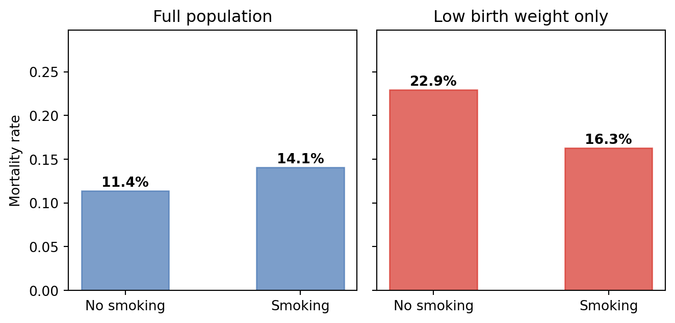

Figure 6: Mortality rates by smoking status, stratified by birth weight. In the full population (left), smoking raises mortality. Among low-birth-weight babies (right), the relationship reverses — conditioning on the collider creates a spurious protective signal.

The correct model

The full structural model includes the causal arrows in Figure 5. We do not condition on birth weight when estimating the total effect of smoking on mortality — pathmc’s structural specification keeps all paths active.

spec_bw = """
birth_weight ~ smoking + birth_defect
mortality ~ b_smoking*smoking + birth_defect
"""

model_bw = pathmc.model(spec_bw, data=df_bw, families={"mortality": "bernoulli"})
model_bw.equations()

\begin{aligned} \beta_{birth,weight} &\sim \text{Normal}(mu=0,\, sigma=10) \\ \sigma_{birth,weight} &\sim \text{HalfNormal}(sigma=1) \\ \beta_{mortality} &\sim \text{Normal}(mu=0,\, sigma=10) \\[6pt] \mu_{birth,weight} &= \beta_{0,\,birth,weight} + \mathrm{smoking} + \mathrm{birth\_defect} \\ \mathrm{birth\_weight} &\sim \text{Normal}(\mu_{birth,weight},\, \sigma_{birth,weight}) \\ \mu_{mortality} &= \beta_{0,\,mortality} + b_{smoking} \cdot \mathrm{smoking} + \mathrm{birth\_defect} \\ \mathrm{mortality} &\sim \text{Bernoulli}(\text{logit}^{-1}(\mu_{mortality})) \end{aligned}

Collider warnings and identification

warnings = model_bw.collider_warnings({"birth_weight"}, "smoking", "mortality")
for w in warnings:
    print(w)

'birth_weight' is a collider between 'smoking' and 'mortality'. Conditioning on it may open a spurious path and introduce bias.

print(f"Identifiable?    {model_bw.is_identifiable('smoking', 'mortality')}")
print(f"Adjustment sets: {model_bw.adjustment_sets('smoking', 'mortality')}")

Identifiable?    True
Adjustment sets: [set()]

model_bw.fit(draws=500, tune=500, chains=4, random_seed=42)

NUTS[nutpie]: [beta_mortality, beta_birth_weight, sigma_birth_weight]

r0 = model_bw.do(set={"smoking": 0.0}, kind="mean")
r1 = model_bw.do(set={"smoking": 1.0}, kind="mean")

ate_bw = r1 - r0
ate_bw

DoResult — 2000 draws, 4 variables

variable	mean	94% HDI
smoking	1.00	[1.00, 1.00]
birth_defect	0.00	[0.00, 0.00]
birth_weight	-0.52	[-0.55, -0.48]
mortality	0.03	[0.01, 0.06]

Methods: .draws() .mean() .hdi() .by_time() .dataset

The ATE is positive — smoking increases mortality, as expected.

The biased analysis

To demonstrate collider bias computationally, we fit a model that uses birth weight and smoking to predict mortality, without accounting for birth defects. By conditioning on birth weight (the collider), this model opens the spurious path smoking - - birth_weight - - birth_defect → mortality.

biased_model = pathmc.model(
    "mortality ~ b_smoking_biased*smoking + birth_weight",
    data=df_bw,
    families={"mortality": "bernoulli"},
)
biased_model.fit(draws=500, tune=500, chains=4, random_seed=42)

NUTS[nutpie]: [beta_mortality]

biased_ate = biased_model.ate("mortality", "smoking", values=(0.0, 1.0))
biased_ate

ATE of smoking on mortality

Mean	-0.05
94% HDI	[-0.07, -0.03]
P(> 0)	0.00
Draws	2000

Methods: .hdi() .prob() .summary() .draws() .by_time() .dataset

Comparing estimates

Figure 7 shows the core result: the correct model recovers the true harmful effect of smoking, while the biased model (conditioning on the collider) attenuates it toward zero or reverses its sign.

Code

fig, ax = plt.subplots(figsize=(FIG_WIDTH, FIG_HEIGHT * 0.65))

correct_val = ate_bw.mean("mortality")
correct_hdi = ate_bw.hdi("mortality", prob=0.94)
biased_val = biased_ate.mean()
biased_hdi = biased_ate.hdi(prob=0.94)

ax.errorbar(
    biased_val,
    1,
    xerr=[[biased_val - biased_hdi[0]], [biased_hdi[1] - biased_val]],
    fmt="o",
    color="C3",
    capsize=5,
    label="Biased (conditions on collider)",
)
ax.errorbar(
    correct_val,
    0,
    xerr=[[correct_val - correct_hdi[0]], [correct_hdi[1] - correct_val]],
    fmt="o",
    color="C0",
    capsize=5,
    label="Correct (full DAG)",
)
ax.axvline(0, color="gray", linestyle=":", alpha=0.5)
ax.set_yticks([0, 1])
ax.set_yticklabels(["Correct model", "Biased model"])
ax.set_xlabel("ATE of smoking on mortality (risk difference)")
ax.legend(loc="best", fontsize=9)
plt.tight_layout()
plt.show()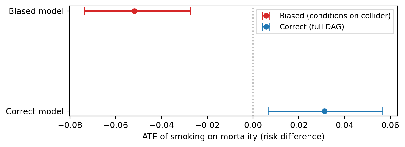

Figure 7: Correct vs biased ATE estimates. The correct model (including birth defects, not conditioning on the collider) recovers the true harmful effect. The biased model (conditioning on birth weight without birth defects) attenuates the effect toward zero.

Collider bias in action

The biased model — which conditions on birth weight without accounting for birth defects — attenuates or reverses the harmful effect of smoking. This is exactly the birth-weight paradox: among babies of similar birth weight, smokers’ babies appear healthier because the non-smoking low-weight babies are more likely to have birth defects.

pathmc’s collider_warnings() catches this before it leads to wrong conclusions.

Every example above had a crucial advantage: the confounders were observed. But what if the confounder cannot be measured?

When backdoor fails: the front-door criterion

A company wants to know whether its advertising causes sales, but an unmeasured confounder — say, seasonal demand — drives both ad spending and sales. With no way to measure the confounder, the backdoor criterion fails. Is identification hopeless?

Not necessarily. If advertising affects sales through a measurable mediator (say, website visits), and that mediator is not directly confounded with sales, Pearl’s front-door criterion (Pearl et al. 2016, sec. 3.4) provides an alternative path to identification.

Figure 8: The advertising scenario as a front-door structure. Seasonal demand (unobserved) confounds ad spend and sales, but website visits mediate the full causal effect of advertising, enabling identification.

The causal structure

The front-door structure has four key features: an unobserved confounder U that blocks backdoor identification, and a mediator M that carries the entire causal effect from X to Y.

Figure 9: Front-door structure: the unobserved confounder U (dashed) blocks backdoor identification of X → Y. But the mediator M satisfies the front-door criterion, enabling identification through the X → M → Y path.

Three conditions make the front-door criterion work (Pearl 2009):

X → M is unconfounded (no backdoor path from X to M)
M → Y is confounded by U, but X blocks all backdoor paths from M to Y
M fully mediates the effect of X on Y (no direct X → Y arrow)

Simulate data

We generate data with a known confounding structure. The true causal effect of X on Y (through M) is a × b = 0.6 × 0.5 = 0.3. The confounder U inflates the naive X → Y association.

n_fd = 1000

U = rng.normal(size=n_fd)
X_fd = 0.7 * U + rng.normal(scale=0.5, size=n_fd)
M_fd = 0.6 * X_fd + rng.normal(scale=0.5, size=n_fd)
Y_fd = 0.5 * M_fd + 0.8 * U + rng.normal(scale=0.5, size=n_fd)

TRUE_INDIRECT = 0.6 * 0.5

df_fd = pd.DataFrame({"X": X_fd, "M": M_fd, "Y": Y_fd})

Notice that U is not in the DataFrame — it is unobserved.

The confounding problem, visualized

Figure 10 shows why a naive analysis fails. The scatter of X vs Y has a steep slope because the confounder U pushes both variables in the same direction. The true causal effect (0.3) is much weaker than the observed association.

Code

from numpy.polynomial.polynomial import polyfit

fig, ax = plt.subplots(figsize=(FIG_WIDTH, FIG_HEIGHT))

scatter = ax.scatter(X_fd, Y_fd, c=U, cmap="viridis", alpha=0.4, s=15, rasterized=True)
cbar = plt.colorbar(scatter, ax=ax, label="Confounder U (unobserved)")

raw_coeffs = polyfit(X_fd, Y_fd, 1)
x_range = np.linspace(X_fd.min(), X_fd.max(), 100)
ax.plot(
    x_range,
    raw_coeffs[0] + raw_coeffs[1] * x_range,
    "--",
    color="gray",
    linewidth=2,
    label=f"Raw slope = {raw_coeffs[1]:.2f} (confounded)",
)
ax.plot(
    x_range,
    np.mean(Y_fd) + TRUE_INDIRECT * (x_range - np.mean(X_fd)),
    "--",
    color="black",
    linewidth=2,
    label=f"True causal slope = {TRUE_INDIRECT} (front-door)",
)

ax.set_xlabel("X")
ax.set_ylabel("Y")
ax.legend(loc="upper left", fontsize=9)
plt.tight_layout()
plt.show()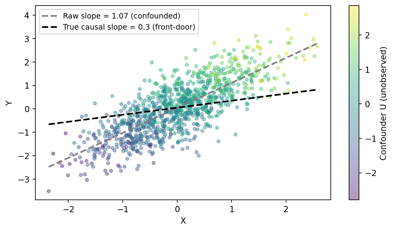

Figure 10: X vs Y colored by the unobserved confounder U. The raw regression slope (gray dashed) is steeper than the true causal effect (black dashed) because U inflates both X and Y.

The naive approach fails

A naive regression of Y on X (ignoring both the mediator and the confounder) gives a biased estimate because the backdoor path X ← U → Y is open.

naive = pathmc.model("Y ~ b_naive*X", data=df_fd)
naive.fit(draws=500, tune=500, chains=4, random_seed=42)

NUTS[nutpie]: [beta_Y, sigma_Y]

naive_ate = naive.ate("Y", "X", values=(0.0, 1.0))
print(f"True indirect effect: {TRUE_INDIRECT:.1f}")
naive_ate

True indirect effect: 0.3

ATE of X on Y

Mean	1.07
94% HDI	[1.02, 1.12]
P(> 0)	1.00
Draws	2000

Methods: .hdi() .prob() .summary() .draws() .by_time() .dataset

The front-door solution: mediation

The key insight: even though U confounds X → Y, the two sub-paths are separately identifiable.

X → M: X is the only cause of M in the DAG, so the X → M coefficient is unconfounded.
M → Y: U confounds this path, but conditioning on X blocks the backdoor M ← X ← U → Y. Since X is observed, the M → Y coefficient conditional on X is identified.

The total causal effect is the product of these two identified coefficients: a × b.

spec_fd = """
M ~ a*X
Y ~ b*M + X
indirect := a*b
"""

model_fd = pathmc.model(spec_fd, data=df_fd)
model_fd.graph()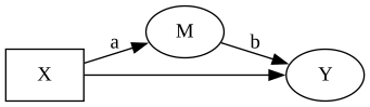

model_fd.equations()

\begin{aligned} \beta_{M} &\sim \text{Normal}(mu=0,\, sigma=10) \\ \sigma_{M} &\sim \text{HalfNormal}(sigma=1) \\ \beta_{Y} &\sim \text{Normal}(mu=0,\, sigma=10) \\ \sigma_{Y} &\sim \text{HalfNormal}(sigma=1) \\[6pt] \mu_{M} &= \beta_{0,\,M} + a \cdot \mathrm{X} \\ \mathrm{M} &\sim \text{Normal}(\mu_{M},\, \sigma_{M}) \\ \mu_{Y} &= \beta_{0,\,Y} + b \cdot \mathrm{M} + \mathrm{X} \\ \mathrm{Y} &\sim \text{Normal}(\mu_{Y},\, \sigma_{Y}) \\ indirect &\equiv a \cdot b \end{aligned}

Why include X in the Y equation?

The regression Y ~ M + X is not about the direct effect of X on Y (there is none in the true DAG). Including X as a covariate in the Y equation blocks the backdoor path from M to Y through U (the path M ← X ← U → Y). Without X in this equation, the b coefficient would absorb confounding from U.

Identification check

The backdoor criterion cannot find an adjustment set for X → Y (there is none — the confounder is unobserved):

print(f"Backdoor identifiable? {model_fd.is_identifiable('X', 'Y')}")
print(f"Adjustment sets:       {model_fd.adjustment_sets('X', 'Y')}")

Backdoor identifiable? True
Adjustment sets:       [set()]

But the front-door criterion can identify the effect through M. Because the estimation spec adds X to the Y equation (an adjustment edge absent from the true causal DAG), we check against a data-free model of the causal structure directly:

causal_model = pathmc.model(
    """
    M ~ X
    Y ~ M
    """
)
identifiable, message = causal_model.frontdoor_identifiable("X", "M", "Y")
print(f"Front-door identifiable? {identifiable}")
print(f"Message: {message}")

Front-door identifiable? True
Message: Front-door criterion satisfied: the causal effect of 'X' on 'Y' is identified through 'M'.

Fit the model

model_fd.fit(draws=500, tune=500, chains=4, random_seed=42)

NUTS[nutpie]: [beta_Y, sigma_M, beta_M, sigma_Y]

model_fd.effects_summary()

	mean	sd	hdi_3%	hdi_97%
name
a	0.595374	0.018677	0.560579	0.630010
b	0.557240	0.042054	0.479106	0.636277
indirect	0.331779	0.027265	0.277947	0.379547

The indirect parameter (a × b) recovers the true causal effect of {TRUE_INDIRECT:.1f} without observing U.

effects = model_fd.effects_summary()
print(f"True indirect effect (a×b): {TRUE_INDIRECT:.1f}")
effects

True indirect effect (a×b): 0.3

	mean	sd	hdi_3%	hdi_97%
name
a	0.595374	0.018677	0.560579	0.630010
b	0.557240	0.042054	0.479106	0.636277
indirect	0.331779	0.027265	0.277947	0.379547

Why not use model.ate("Y", "X") here?

The do(X) operator performs graph surgery on the structural equations as written. Because the spec includes X in the Y equation (Y ~ b*M + X), do(X) propagates the intervention through both the mediated path (X → M → Y) and the X coefficient in the Y equation. But that X coefficient is not a causal effect — it is a confounding proxy for U, included only to block the backdoor path from M to Y. The do() operator cannot distinguish adjustment variables from causal arrows.

For the front-door criterion, the correct estimate is the defined parameter indirect := a*b, which computes the product of the two identified path coefficients.

Comparing approaches

Figure 11 summarizes the core result: the naive regression overshoots because of confounding, while the front-door indirect effect a × b recovers the true causal effect.

Code

fig, ax = plt.subplots(figsize=(FIG_WIDTH, FIG_HEIGHT * 0.65))

naive_val = naive_ate.mean()
naive_hdi = naive_ate.hdi(prob=0.94)
fd_effect = effects.loc["indirect"]
fd_mean = fd_effect["mean"]
fd_hdi_low = fd_effect["hdi_3%"]
fd_hdi_high = fd_effect["hdi_97%"]

ax.errorbar(
    naive_val,
    1,
    xerr=[[naive_val - naive_hdi[0]], [naive_hdi[1] - naive_val]],
    fmt="o",
    color="C3",
    capsize=5,
    label="Naive (confounded)",
)
ax.errorbar(
    fd_mean,
    0,
    xerr=[[fd_mean - fd_hdi_low], [fd_hdi_high - fd_mean]],
    fmt="o",
    color="C0",
    capsize=5,
    label="Front-door (indirect a×b)",
)
ax.axvline(
    TRUE_INDIRECT,
    color="black",
    linestyle="--",
    label=f"True causal effect ({TRUE_INDIRECT})",
)
ax.set_yticks([0, 1])
ax.set_yticklabels(["Front-door", "Naive"])
ax.set_xlabel("ATE of X on Y")
ax.legend(loc="best", fontsize=9)
plt.tight_layout()
plt.show()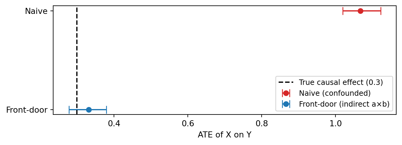

Figure 11: Naive regression vs front-door indirect effect. The naive estimate (confounded by U) overestimates the causal effect. The front-door mediation model recovers the true effect of 0.3 via the indirect path a × b. Black dashed line marks the true DGP value.

When does the front-door criterion apply?

The front-door criterion requires a specific DAG structure (Pearl et al. 2016, sec. 3.4):

Complete mediation: X affects Y only through M (no direct X → Y edge).
No X → M confounding: there is no unobserved common cause of X and M.
M → Y confounding is blocked by X: conditioning on X closes all backdoor paths from M to Y.

These conditions are strong and may not hold in many applied settings. But when they do hold, the front-door criterion identifies the causal effect even with unmeasured confounding of X and Y.

From front-door to mediation

In pathmc, the front-door criterion is implemented naturally as mediation analysis: label the path coefficients, define the indirect effect with :=, and let the structural model handle identification. This means you don’t need a separate “front-door estimator” — the same tools used for mediation analysis apply here.

Summary

Confounders (common causes) must be adjusted for. .adjustment_sets() identifies them.
Mediators are descendants of treatment — they are automatically excluded from backdoor sets. Conditioning on them when estimating the total effect blocks the causal path and introduces bias.
Colliders must not be adjusted for. .collider_warnings() flags them.
.is_identifiable() tells you whether any valid backdoor adjustment set exists before you run a single MCMC sample.
Collider bias is created by analysis choices, not present in the raw data. The birth-weight paradox (Section 6) demonstrates how conditioning on a collider can reverse a harmful effect, making smoking appear protective among low-birth-weight babies.
Unmeasured confounding blocks the backdoor criterion, but the front-door criterion (Section 7) can still identify the effect when all causal paths flow through a measured mediator. .frontdoor_identifiable() checks the three required conditions.
The DAG encodes your assumptions. pathmc’s identification helpers check the logical consequences of those assumptions, but the DAG itself must come from domain knowledge.

Reflection

Which variables in your analysis might be colliders — or unmeasured confounders?

Collider trap: “customer satisfaction” is caused by both product quality and marketing — conditioning on it when estimating the effect of marketing on retention could introduce collider bias.
Front-door opportunity: if a confounder is unmeasured but the treatment affects the outcome entirely through a measurable mediator (e.g. ad spend → clicks → purchases, with seasonal demand confounding ad spend and purchases), the front-door criterion may rescue identification.
Hiring: “Top university” and “strong portfolio” both cause “getting hired.” Among hired employees, university prestige and portfolio quality will appear negatively correlated — conditioning on the collider.

References

Hernández-Díaz, Sonia, Enrique F. Schisterman, and Miguel A. Hernán. 2006. “The Birth Weight ‘Paradox’ Uncovered?” American Journal of Epidemiology 164 (11): 1115–20. https://doi.org/10.1093/aje/kwj275.

Pearl, Judea. 2009. Causality: Models, Reasoning, and Inference. 2nd ed. Cambridge University Press.

Pearl, Judea, Madelyn Glymour, and Nicholas P. Jewell. 2016. Causal Inference in Statistics: A Primer. John Wiley & Sons.

Pearl, Judea, and Dana Mackenzie. 2018. The Book of Why: The New Science of Cause and Effect. Basic Books.