Counterfactuals: From Population to Individual

Interventions tell us what happens on average when we force a change. Counterfactuals answer a different question: what would have happened to this specific person under different circumstances?

Author

Benjamin Vincent

A student named Joe participates in an after-school remedial program. We observe his encouragement level (X = 0.5), his homework hours (H = 1), and his exam score (Y = 1.5 standard deviations above the mean). His teacher asks: “What would Joe’s score have been had he doubled his homework?”

This is not a population-level question — “what happens on average when we set homework to 2?” — it is a question about one specific individual whose characteristics we have already observed. The answer depends on Joe’s personal traits, not the population average.

Pearl calls this a counterfactual (Pearl et al. 2016, sec. 4.2.3): a statement about what would have happened under conditions that did not actually occur, for a specific unit whose factual outcome is known. The do() operator cannot answer this question because it averages over all individuals. Counterfactuals require an additional step — using Joe’s observed data to infer his individual characteristics before simulating the hypothetical scenario.

The encouragement design

The example comes from an “encouragement design” (Pearl et al. 2016, sec. 4.2.3): a randomized pilot program where students are assigned to remedial sessions by lottery. Three variables, all standardized to mean 0 and variance 1:

X — encouragement (time in the after-school program)
H — homework (hours spent studying)
Y — exam score

Figure 1: Encouragement design. X (encouragement) affects Y (exam score) directly and indirectly through H (homework). All exogenous factors (U) are independent — this is a randomized design with no confounding.

The structural equations are:

\begin{aligned} X &= U\_X \\ H &= a \cdot X + U\_H \\ Y &= b \cdot X + c \cdot H + U\_Y \end{aligned}

with a = 0.5, b = 0.7, c = 0.4, and all U terms mutually independent. Because encouragement is randomized, X has no structural parents — it is determined entirely by the exogenous factor U_X.

The U terms will turn out to be the key to answering Joe’s counterfactual question. Their interpretation is different from what you may expect if you’re used to thinking of residuals as noise — we’ll return to this after seeing what the do() operator can and cannot tell us.

Simulate data

We generate a large sample from the known data-generating process so that the Bayesian model can recover the true coefficients precisely.

import numpy as np
import pandas as pd
import pathmc

rng = np.random.default_rng(42)
n = 2000

TRUE_A = 0.5
TRUE_B = 0.7
TRUE_C = 0.4

U_X = rng.normal(size=n)
U_H = rng.normal(size=n)
U_Y = rng.normal(size=n)

X = U_X
H = TRUE_A * X + U_H
Y = TRUE_B * X + TRUE_C * H + U_Y

df = pd.DataFrame({"X": X, "H": H, "Y": Y})
df.head()

	X	H	Y
0	0.304717	-0.299592	0.346669
1	-1.039984	-1.185870	-0.307118
2	0.750451	0.809235	1.122331
3	0.940565	0.722137	3.186082
4	-1.951035	-2.380309	-0.888061

Fit the structural model

spec = """
H ~ a*X
Y ~ b*X + c*H
"""

model = pathmc.model(spec, data=df)
model.graph()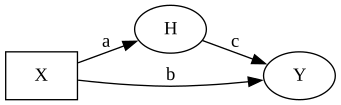

model.equations()

\begin{aligned} \beta_{H} &\sim \text{Normal}(mu=0,\, sigma=10) \\ \sigma_{H} &\sim \text{HalfNormal}(sigma=1) \\ \beta_{Y} &\sim \text{Normal}(mu=0,\, sigma=10) \\ \sigma_{Y} &\sim \text{HalfNormal}(sigma=1) \\[6pt] \mu_{H} &= \beta_{0,\,H} + a \cdot \mathrm{X} \\ \mathrm{H} &\sim \text{Normal}(\mu_{H},\, \sigma_{H}) \\ \mu_{Y} &= \beta_{0,\,Y} + b \cdot \mathrm{X} + c \cdot \mathrm{H} \\ \mathrm{Y} &\sim \text{Normal}(\mu_{Y},\, \sigma_{Y}) \end{aligned}

idata = model.fit(draws=1000, tune=1000, chains=4, random_seed=42)

NUTS[nutpie]: [sigma_H, beta_H, beta_Y, sigma_Y]

The recovered coefficients should be close to the true values (a = 0.5, b = 0.7, c = 0.4):

model.effects_summary()

	mean	sd	hdi_3%	hdi_97%
name
a	0.505260	0.022287	0.464623	0.547927
b	0.671924	0.025281	0.626583	0.720277
c	0.445056	0.022237	0.400882	0.484564

The population-level question: do(H = 2)

Before we tackle Joe’s counterfactual, consider the population-level interventional question: “What would happen to the average exam score if we forced every student’s homework to 2?”

The do() operator performs graph surgery — it severs all arrows into H and fixes H = 2 for every student. Since the DGP is standardized (mean 0), the population has average X \approx 0 and average U_Y \approx 0:

E[Y \mid do(H = 2)] = b \cdot E[X] + c \cdot 2 + E[U_Y] \approx 0.7 \cdot 0 + 0.4 \cdot 2 + 0 = 0.8

do_result = model.do(set={"H": 2.0})
print("Expected: E[Y | do(H=2)] ≈ 0.8")
do_result

Expected: E[Y | do(H=2)] ≈ 0.8

DoResult — 4000 draws, 3 variables

variable	mean	94% HDI
X	-0.06	[-0.06, -0.06]
H	2.00	[2.00, 2.00]
Y	0.87	[0.77, 0.96]

Methods: .draws() .mean() .hdi() .by_time() .dataset

This is a valid causal quantity, but it answers the wrong question for Joe. The do-operator tells us about the average student under the intervention, not about Joe specifically. Joe is not average — he has above-average encouragement (X = 0.5 > 0) and (as we will see) above-average inherent exam ability.

The residual is not noise

If you come from a Bayesian or frequentist statistics background, you probably read the U terms in the structural equations as noise — zero-mean, normally distributed error terms that represent the part of the data your model can’t explain. In standard regression, the residual for observation i is exchangeable with every other residual. You wouldn’t try to “preserve” a specific individual’s residual, because it carries no meaningful information — it’s just estimation error.

In a structural causal model, the U terms play a fundamentally different role. They look like regression residuals — across the population, they’re zero-mean and normally distributed. But for any specific individual, U_Y encodes everything about that person that causally affects Y but isn’t captured by the measured variables.

For Joe, U_Y = 0.75 is not noise. It is his natural test-taking ability, his sleep quality the night before, his intrinsic motivation, his breakfast that morning — every unmeasured factor that pushes his exam score above what his encouragement and homework levels alone would predict. These are real causal inputs, not estimation artifacts. The structural equation Y = b \cdot X + c \cdot H + U_Y says: “Joe’s exam score is determined by his encouragement, his homework, and everything else about Joe that matters.”

This reinterpretation — from “discardable error” to “signal about the individual” — is the conceptual shift that enables counterfactual reasoning.

The dual nature of U

Across the population, U_Y behaves like noise: U_Y \sim \text{Normal}(0, \sigma), independent of the other variables. This is why fitting the model with standard regression works perfectly well.

For a specific individual, U_Y is a fixed property — it characterizes everything about that person that the model doesn’t measure. Two students with the same X and H can have different exam scores because they have different U_Y values, which reflect genuinely different (but unmeasured) causal factors.

The same quantity plays both roles, and which interpretation matters depends on whether you’re asking a population question or an individual one.

Why holding U fixed makes sense

When we ask “what would Joe’s score have been with more homework?”, we’re asking about a hypothetical change to one variable while keeping everything else about Joe the same. Changing Joe’s homework doesn’t change his innate ability, his sleep quality, or his motivation — those are properties of Joe, not consequences of his homework level. In the structural model, this means U_Y stays fixed at 0.75 when we hypothetically set H = 2.

This is exactly what the do() operator doesn’t do. When pathmc computes do(H = 2), it uses the population mean for all exogenous variables: U_Y \approx 0, X \approx 0. That’s correct for a policy question (“what happens to the average student?”) but wrong for a counterfactual about Joe, because it replaces Joe’s actual characteristics with the average person’s.

The link to posterior predictive checks

If you’ve done Bayesian modeling, this distinction might remind you of the difference between:

Posterior predictive for a new observation: “What score would a new, random student get if we set their homework to 2?” — uses U_Y \sim \text{Normal}(0, \sigma), averaging over possible individuals.
Posterior predictive for a specific, observed individual: “What score would Joe get if we changed his homework to 2, given that we’ve already observed his actual score?” — requires conditioning on Joe’s data first to infer his U_Y.

Standard Bayesian prediction doesn’t typically make this second move, because in a pure prediction context there’s no reason to — the residual really is just noise. But when the model represents causal mechanisms, the residual carries individual-level information that matters for counterfactual questions. The abduction step (inferring U_Y from Joe’s data) is what bridges prediction and counterfactual reasoning.

The counterfactual question: what about Joe?

Joe’s observed values are X = 0.5, H = 1, Y = 1.5. We want to know what his score would have been had he doubled his homework to H = 2, keeping everything else about Joe — his encouragement level, his inherent ability, his other personal characteristics — fixed.

Now the logic should be clear: we need to (1) recover Joe’s personal U values from his observed data, (2) modify the model to set H = 2, and (3) predict Joe’s score in the modified model using his personal U values — not the population average.

The three-step procedure

Pearl’s three-step procedure for computing counterfactuals (Pearl et al. 2016, sec. 4.2.4):

Abduction — Use Joe’s observed data to infer his exogenous characteristics (U values).
Action — Modify the model: replace the equation for H with H = 2.
Prediction — Compute Y in the modified model using Joe’s U values.

Step 1: Abduction

From the structural equations and Joe’s data (X = 0.5, H = 1, Y = 1.5):

\begin{aligned} U\_X &= X = 0.5 \\ U\_H &= H - a \cdot X = 1 - 0.5 \times 0.5 = 0.75 \\ U\_Y &= Y - b \cdot X - c \cdot H = 1.5 - 0.7 \times 0.5 - 0.4 \times 1 = 0.75 \end{aligned}

Joe’s U_H and U_Y are both 0.75 — he has above-average inherent homework effort and above-average inherent exam ability, independent of the encouragement program.

Step 2: Action

Replace the homework equation H = a \cdot X + U_H with the constant H = 2.

Step 3: Prediction

Compute Y in the modified model:

Y_{H=2} = b \cdot X + c \cdot 2 + U_Y = 0.7 \times 0.5 + 0.4 \times 2 + 0.75 = 0.35 + 0.8 + 0.75 = 1.90

Joe’s score would have been 1.90 standard deviations above the mean, instead of his observed 1.50.

A simpler form

Since only H changes and X stays fixed at Joe’s observed value, the counterfactual simplifies:

Y_{H=2} - Y_{\text{obs}} = c \cdot (H_{\text{new}} - H_{\text{obs}}) = 0.4 \times (2 - 1) = 0.4

The counterfactual increase depends only on the direct H \to Y coefficient. The other pathways (X \to Y, the U terms) cancel out because they are unchanged by the intervention on H.

What’s happening under the hood: manual implementation

With real data, we don’t know the true coefficients — we have posterior distributions over them. The three-step procedure extends naturally: for each posterior draw d, compute Joe’s counterfactual using that draw’s coefficient values.

JOE_X = 0.5
JOE_H = 1.0
JOE_Y = 1.5
H_NEW = 2.0

a_draws = idata.posterior["beta_H"].sel(H_predictors="X").values.flatten()
b_draws = idata.posterior["beta_Y"].sel(Y_predictors="X").values.flatten()
c_draws = idata.posterior["beta_Y"].sel(Y_predictors="H").values.flatten()
intercept_H = idata.posterior["beta_H"].sel(H_predictors="Intercept").values.flatten()
intercept_Y = idata.posterior["beta_Y"].sel(Y_predictors="Intercept").values.flatten()

Abduction: infer Joe’s exogenous characteristics from the fitted model.

u_h = JOE_H - intercept_H - a_draws * JOE_X
u_y = JOE_Y - intercept_Y - b_draws * JOE_X - c_draws * JOE_H

print(f"U_H posterior mean: {u_h.mean():.3f}  (analytical = 0.75)")
print(f"U_Y posterior mean: {u_y.mean():.3f}  (analytical = 0.75)")

U_H posterior mean: 0.731  (analytical = 0.75)
U_Y posterior mean: 0.706  (analytical = 0.75)

Action + Prediction: replace H = 2 and compute Y.

y_counterfactual = intercept_Y + b_draws * JOE_X + c_draws * H_NEW + u_y

import arviz as az

y_cf_mean = y_counterfactual.mean()
y_cf_hdi = az.hdi(y_counterfactual, prob=0.94)

print("Joe's counterfactual score (H → 2)")
print(f"  Posterior mean:  {y_cf_mean:.3f}   (analytical = 1.90)")
print(f"  94% HDI:         [{y_cf_hdi[0]:.3f}, {y_cf_hdi[1]:.3f}]")

Joe's counterfactual score (H → 2)
  Posterior mean:  1.945   (analytical = 1.90)
  94% HDI:         [1.901, 1.985]

The posterior mean lands close to the analytical result of 1.90. The HDI reflects uncertainty in the coefficient c — with enough data, this interval shrinks around the true value.

The counterfactual API

The manual implementation above shows exactly what pathmc does internally. The same computation is available as a single method call — no need to know parameter naming conventions or implement abduction yourself:

cf_result = model.counterfactual(
    evidence={"X": JOE_X, "H": JOE_H, "Y": JOE_Y},
    do={"H": H_NEW},
)
print("Joe's counterfactual score (H → 2)")
print(f"  Posterior mean:  {cf_result.mean('Y'):.3f}   (analytical = 1.90)")
print(f"  94% HDI:         {cf_result.hdi('Y', prob=0.94)}")

Joe's counterfactual score (H → 2)
  Posterior mean:  1.945   (analytical = 1.90)
  94% HDI:         [1.90088156 1.98456449]

The API returns a DoResult with the same .mean(), .hdi(), and contrast interface as model.do().

Note

This release supports fully observed, cross-sectional Gaussian linear SEMs. Panel models, latent variables, non-Gaussian families, and transform or lag terms are not yet supported.

Counterfactual contrasts are valid only between counterfactuals computed from identical evidence; do not contrast a counterfactual with a population-level do() result.

This is not pm.observe + pm.do

Counterfactuals operate across two worlds that share exogenous variables but differ in their structural equations. In the factual world, Joe’s observed Y = 1.5 is evidence used to infer his U_Y. In the counterfactual world, Y is the output we want to predict. You cannot express this as a single pm.observe(Y=1.5) + pm.do(H=2) call — observation conditions Y in the generative model, but counterfactuals need the original equation for abduction and a modified equation for prediction. The counterfactual() method implements this two-pass logic directly on posterior draws.

Population intervention vs individual counterfactual

Code

import matplotlib.pyplot as plt

FIG_WIDTH = 7
FIG_HEIGHT = 4

fig, ax = plt.subplots(figsize=(FIG_WIDTH, FIG_HEIGHT * 0.75))

COLOR_POP = "C3"
COLOR_JOE = "C0"

do_val = do_result.mean("Y")
do_hdi = do_result.hdi("Y", prob=0.94)
y_cf_mean = cf_result.mean("Y")
y_cf_hdi = cf_result.hdi("Y", prob=0.94)

ax.errorbar(
    do_val,
    1,
    xerr=[[do_val - do_hdi[0]], [do_hdi[1] - do_val]],
    fmt="o",
    color=COLOR_POP,
    capsize=5,
    markersize=8,
    label="Population: E[Y | do(H=2)]",
)
ax.errorbar(
    y_cf_mean,
    0,
    xerr=[[y_cf_mean - y_cf_hdi[0]], [y_cf_hdi[1] - y_cf_mean]],
    fmt="s",
    color=COLOR_JOE,
    capsize=5,
    markersize=8,
    label=r"Joe: $Y_{H=2}$ (counterfactual)",
)

ax.axvline(0.8, color=COLOR_POP, linestyle="--", alpha=0.5, linewidth=1)
ax.axvline(1.90, color=COLOR_JOE, linestyle="--", alpha=0.5, linewidth=1)

ax.set_yticks([0, 1])
ax.set_yticklabels([r"Joe's counterfactual ($Y_{H=2}$)", "Population do(H=2)"])
ax.set_xlabel("Exam score (standard deviations above mean)")
ax.legend(loc="lower right", fontsize=9)
plt.tight_layout()
plt.show()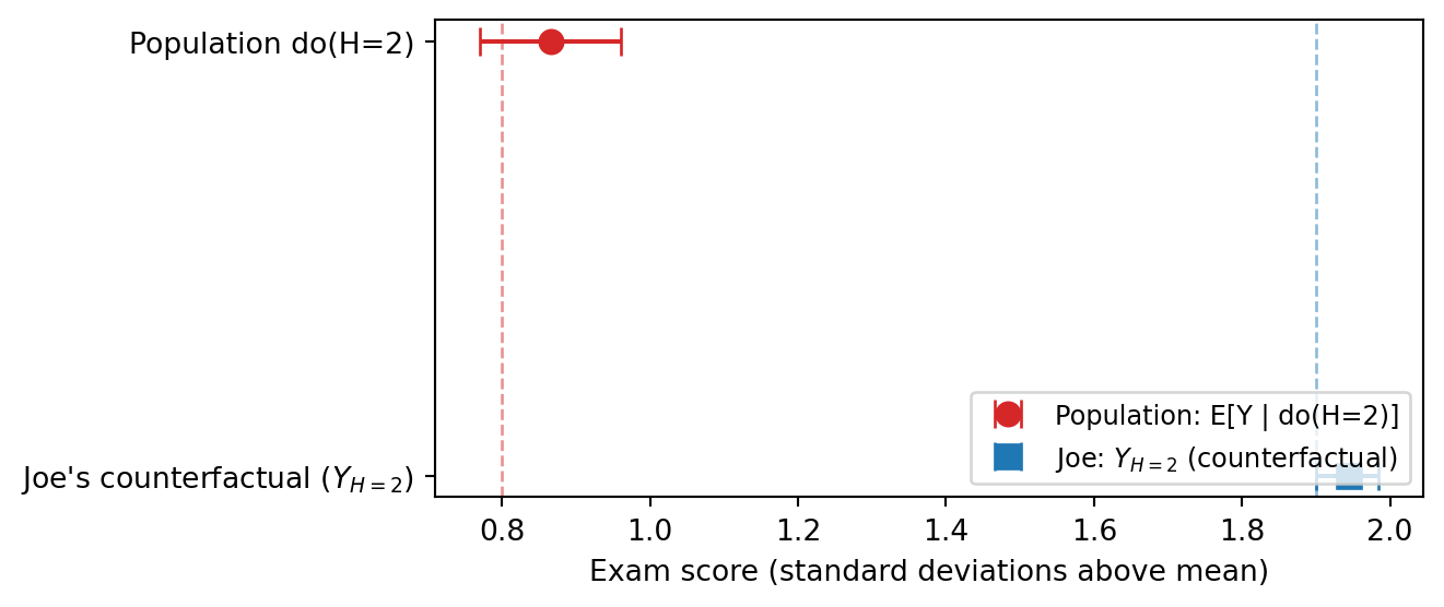

Figure 2: Population-level intervention E[Y | do(H=2)] vs Joe’s individual counterfactual Y_{H=2}. The do-operator predicts the average outcome across all students; the counterfactual uses Joe’s specific characteristics to predict his personal outcome. Black dashed lines mark the analytical values.

The gap between the two estimates reflects the difference between asking about the average person versus asking about Joe specifically. Joe’s counterfactual score is higher because the abduction step reveals that Joe has above-average U_X and U_Y — characteristics that the population-level do-operator averages away.

The counterfactual posterior

Figure 3 shows the full posterior distribution over Joe’s counterfactual score. The distribution is narrow because the coefficient c is well-identified with 2000 observations, but smaller samples or weaker identification would produce greater uncertainty.

Code

fig, ax = plt.subplots(figsize=(FIG_WIDTH, FIG_HEIGHT * 0.75))

x_kde, y_kde, _ = az.kde(cf_result.draws("Y"))
ax.plot(x_kde, y_kde, color=COLOR_JOE, lw=2)
ax.fill_between(x_kde, y_kde, alpha=0.6, color=COLOR_JOE)
ax.axvline(
    1.90,
    color="black",
    linestyle="--",
    linewidth=1.5,
    label="Analytical counterfactual (1.90)",
)
ax.axvline(
    JOE_Y,
    color="gray",
    linestyle="--",
    linewidth=1.5,
    label=f"Observed score ({JOE_Y})",
)
ax.set_xlabel(r"$Y_{H=2}$ (Joe's counterfactual score)")
ax.set_ylabel("Density")
ax.legend(fontsize=9)
plt.tight_layout()
plt.show()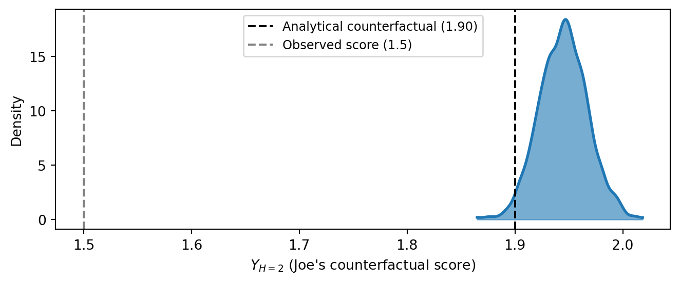

Figure 3: Posterior distribution of Joe’s counterfactual exam score under H = 2. The analytical answer (1.90, black dashed) falls within the posterior. Joe’s observed score (1.50, gray dashed) provides a reference for the counterfactual improvement.

Why interventions and counterfactuals differ

	Intervention: E[Y \mid do(H=2)]	Counterfactual: Y_{H=2} for Joe
Question	What happens on average if we set everyone’s homework to 2?	What would Joe’s score have been if he had done homework H = 2?
Uses individual data?	No — averages over the population	Yes — conditions on Joe’s observed (X, H, Y)
Exogenous values	Population mean (U \approx 0)	Joe’s inferred values (U_Y = 0.75)
Result	\approx 0.80	\approx 1.90

The do() operator is the right tool for policy questions (“should we mandate 2 hours of homework?”). Counterfactuals are the right tool for individual reasoning (“how much would this student have benefited?”), credit assignment, and retrospective evaluation.

Counterfactuals in linear SEMs

In a linear SEM with known coefficients, individual counterfactuals reduce to a closed-form expression. When we intervene on H while keeping all other variables’ equations intact:

Y_{H=h'} = Y_{\text{obs}} + c \cdot (h' - H_{\text{obs}})

The counterfactual change depends only on the direct effect of the intervened variable (c) and the size of the hypothetical change (h' - H_{\text{obs}}). All other structural relationships cancel because they are unchanged by the intervention.

Summary

The U terms are not noise — they are everything about a specific individual that causally affects the outcome but isn’t measured. Across the population, they behave like zero-mean residuals; for a specific person, they encode real, fixed characteristics. This reinterpretation is the conceptual foundation of counterfactual reasoning.
Counterfactuals answer questions about specific individuals under hypothetical conditions — “what would have happened to this person?” — by conditioning on observed evidence before intervening (Pearl et al. 2016, sec. 4.2.3).
Pearl’s three-step procedure — abduction, action, prediction — turns a structural causal model into a counterfactual engine. The abduction step recovers the individual’s U values from their observed data; the prediction step holds those values fixed while simulating the hypothetical change.
do() answers a different question: the population-level average effect of an intervention, using U \approx 0 (the average person). For Joe, do(H = 2) predicts a score of \approx 0.8; the counterfactual predicts \approx 1.9 — the gap is entirely due to Joe’s above-average U values.
model.counterfactual() wraps the three-step procedure in a single call, returning a DoResult with the same interface as do().
In linear SEMs, the counterfactual simplifies: the change in Y equals the direct effect coefficient times the change in the intervened variable, because all other pathways cancel.

Reflection

When have you wanted to answer a question about a specific case rather than a population average?

Medicine: A patient took drug A and recovered slowly. Would drug B have worked better for this patient, given their age, comorbidities, and biomarkers?
Marketing: A customer saw ad campaign A and didn’t convert. Would they have converted under campaign B, given their browsing history and demographics?
Education: A student attended tutoring sessions but still struggled. Would a different teaching method have helped this student, given their prior performance and engagement level?

In each case, the population-level treatment effect is not enough — you need the individual’s observed data to condition on before asking the counterfactual “what if?”

References

Pearl, Judea, Madelyn Glymour, and Nicholas P. Jewell. 2016. Causal Inference in Statistics: A Primer. John Wiley & Sons.