The House: Which Nodes Must You Adjust For?

A LinkedIn causal-inference puzzle worked end to end in pathmc — read the unique valid adjustment set straight off the DAG, then confirm that adjusting for a confounder helps while adjusting for sinks of the mediator or the outcome wrecks the estimate.

Author

Benjamin Vincent

A puzzle posed by Guénolé Le Pennec, PhD, on LinkedIn asks a deceptively simple question on a seven-node DAG he nicknames “the house”. We want the effect of X1 on X3, and we are asked: which node(s) must be adjusted for, which can be adjusted for, and which must be avoided?

The puzzle ships with R code that fills the house with data and runs five regressions, eyeballing the coefficient on X1 against the known truth (the structural coefficients make the true effect 3 × 2 = 6). This notebook answers the question the way pathmc is designed to: read the answer off the DAG before touching the data with adjustment_sets(), then confirm each verdict by fitting the corresponding model and watching the estimate land on — or fall away from — the true value of 6.

The house

The original data-generating process, transcribed from the puzzle’s R code, has one root (X0) and six structural equations:

Equation	Role of the left-hand side
`X1 = 2·X0 + ε`	treatment, also a child of `X0`
`X2 = 3·X1 + 3 + ε`	mediator on the `X1 → X3` path
`S1 = X1 + 2 + ε`	sink (child of the treatment)
`X3 = 2·X2 − 1.4·X0 + ε`	outcome
`S2 = −2·X2 + 1.3 + ε`	sink (child of the mediator)
`S3 = 1.3·X3 − 2 + ε`	sink (child of the outcome)

Drawn out, the arrows form the house: X0 sits at the apex feeding both X1 and X3, the causal effect runs down the left wall X1 → X2 → X3, and the three S nodes hang off as sinks.

Figure 1: “The house.” X0 (orange) is a common cause of treatment X1 and outcome X3 — the confounder. The causal effect flows X1 → X2 → X3, so X2 (blue) is a mediator. S1, S2, S3 (grey) are sinks: childless descendants of the treatment, mediator, and outcome respectively.

Setup

We simulate from the exact equations above, keeping the original n = 100000 so the Bayesian estimates line up with the lm() coefficients in the puzzle’s R code. The structural model is then a one-to-one transcription of the house.

import numpy as np
import pandas as pd
import matplotlib.pyplot as plt
import pathmc

rng = np.random.default_rng(42)
n = 100_000

X0 = rng.normal(0, 1, n)
X1 = 2 * X0 + rng.normal(0, 1, n)
X2 = 3 * X1 + 3 + rng.normal(0, 1, n)
S1 = X1 + 2 + rng.normal(0, 1, n)
X3 = 2 * X2 - 1.4 * X0 + rng.normal(0, 1, n)
S2 = -2 * X2 + 1.3 + rng.normal(0, 1, n)
S3 = 1.3 * X3 - 2 + rng.normal(0, 1, n)

df = pd.DataFrame({
    "X0": X0,
    "X1": X1,
    "X2": X2,
    "X3": X3,
    "S1": S1,
    "S2": S2,
    "S3": S3,
})

TRUE_EFFECT = 6.0  # 3 (X1 -> X2) * 2 (X2 -> X3)

FIG_WIDTH = 7
FIG_HEIGHT = 4

The structural model is a direct transcription of the house — one regression per endogenous variable, with X0 left exogenous:

spec = """
X1 ~ X0
X2 ~ X1
S1 ~ X1
X3 ~ X2 + X0
S2 ~ X2
S3 ~ X3
"""

house = pathmc.model(spec, data=df)
house.graph()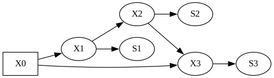

Reading the answer off the DAG

The whole point of a structural model is that the adjustment question is settled by the graph, not by trial and error. pathmc’s is_identifiable() confirms a valid backdoor adjustment exists, and adjustment_sets() enumerates the minimal sets that work.

print(f"Identifiable?    {house.is_identifiable('X1', 'X3')}")
print(f"Adjustment sets: {house.adjustment_sets('X1', 'X3')}")

Identifiable?    True
Adjustment sets: [{'X0'}]

There is exactly one minimal valid adjustment set: {X0}. That single result answers all three parts of the puzzle.

Must adjust for X0. It is a common cause of X1 and X3, opening the backdoor path X1 ← X0 → X3. Leaving it open mixes confounding into the estimate; it appears in the only valid set.
Must avoid X2, S2, S3. Every one of these is a descendant of the treatment, and the backdoor criterion forbids conditioning on descendants of the treatment. X2 is the mediator (blocking it severs the causal path), S2 is a noisy proxy for that mediator, and S3 is a proxy for the outcome. None can appear in a valid set.
Can adjust for S1 (but needn’t). S1 is also a descendant of X1, so it is excluded from the minimal valid set — yet it is a harmless leaf: it sits on no path between X1 and X3 and is not a collider. Conditioning on it neither opens nor closes any relevant path, so it leaves the estimate unbiased while adding nothing.

Why the puzzle’s bias is not collider bias

A natural reflex is to reach for collider_warnings(). Here it stays silent for every candidate — and correctly so:

for adj in [{"X0"}, {"X0", "S1"}, {"X0", "S2"}, {"X0", "S3"}]:
    print(adj, "->", house.collider_warnings(adj, "X1", "X3") or "no collider warning")

{'X0'} -> no collider warning
{'X0', 'S1'} -> no collider warning
{'S2', 'X0'} -> no collider warning
{'X0', 'S3'} -> no collider warning

S2 and S3 are not colliders, so conditioning on them is not collider bias. The damage they do is a different mechanism — conditioning on a descendant of the mediator or of the outcome — and the backdoor criterion already rules them out by excluding all descendants of the treatment. That is exactly why adjustment_sets() is the right tool for this puzzle: a single rule (“no descendants of the treatment”) disqualifies X2, S1, S2, and S3 in one stroke, and the path analysis keeps X0.

A note on sampling speed

Fitting the models below at n = 100000 is slow — roughly a minute or two each. The culprit is the posterior geometry, not the data size alone: several equations have high-variance, non-zero-mean predictors (X2, X3), which make the joint posterior ill-conditioned and force the NUTS sampler into deep, expensive trajectories. We keep n = 100000 here for faithfulness to the original puzzle. Speeding this up — and understanding why obvious fixes such as mean-centering the predictors do not help the coupled model — is on our TODO list (see issue #230).

Confirming each verdict by fitting

The puzzle’s R code runs five regressions of X3 on X1 plus a candidate adjustment set and reads the coefficient on X1. We mirror each one with a one-equation pathmc model, labelling the treatment coefficient b so it surfaces directly in effects_summary() — the Bayesian analogue of lm(...)$coef["X1"], now with full posterior uncertainty.

adjustment_specs = {
    "no adjustment": "X3 ~ b*X1",
    "+ X0  (confounder)": "X3 ~ b*X1 + X0",
    "+ X0 + S1  (sink of X1)": "X3 ~ b*X1 + X0 + S1",
    "+ X0 + S2  (sink of X2)": "X3 ~ b*X1 + X0 + S2",
    "+ X0 + S3  (sink of X3)": "X3 ~ b*X1 + X0 + S3",
}

results = {}
for name, s in adjustment_specs.items():
    m = pathmc.model(s, data=df)
    m.fit(draws=500, tune=500, chains=2, random_seed=42, progressbar=False)
    summary = m.effects_summary().loc["b"]
    results[name] = (summary["mean"], summary["hdi_3%"], summary["hdi_97%"])

table = pd.DataFrame({
    k: {"estimate": v[0], "hdi_3%": v[1], "hdi_97%": v[2]} for k, v in results.items()
}).T
table.round(3)

NUTS[nutpie]: [beta_X3, sigma_X3]
NUTS[nutpie]: [beta_X3, sigma_X3]
NUTS[nutpie]: [beta_X3, sigma_X3]
NUTS[nutpie]: [beta_X3, sigma_X3]
NUTS[nutpie]: [beta_X3, sigma_X3]

	estimate	hdi_3%	hdi_97%
no adjustment	5.442	5.436	5.448
+ X0 (confounder)	6.015	6.002	6.028
+ X0 + S1 (sink of X1)	6.016	5.996	6.033
+ X0 + S2 (sink of X2)	1.219	1.197	1.244
+ X0 + S3 (sink of X3)	0.641	0.629	0.651

The pattern is unambiguous, and it matches the puzzle’s R output line for line:

No adjustment lands near 5.4 — biased, because the open backdoor X1 ← X0 → X3 leaks confounding into the coefficient.
+ X0 snaps to ≈ 6: blocking the one backdoor path identifies the effect. This is the required adjustment.
+ X0 + S1 stays at ≈ 6: adding the harmless treatment sink changes nothing. S1 can be adjusted for.
+ X0 + S2 collapses toward ≈ 1: conditioning on a proxy of the mediator X2 partially blocks the causal path X1 → X2 → X3, destroying most of the effect.
+ X0 + S3 collapses toward ≈ 0.6: conditioning on a descendant of the outcome bleeds away the outcome’s variation. Both S2 and S3 must be avoided.

Code

fig, ax = plt.subplots(figsize=(FIG_WIDTH, FIG_HEIGHT))

labels = list(results.keys())
colors = ["#d73027", "#1a9850", "#1a9850", "#d73027", "#d73027"]
ypos = np.arange(len(labels))[::-1]

for y, (label, color) in zip(ypos, zip(labels, colors)):
    mean, lo, hi = results[label]
    ax.errorbar(
        mean,
        y,
        xerr=[[mean - lo], [hi - mean]],
        fmt="o",
        color=color,
        capsize=4,
        markersize=7,
    )

ax.axvline(TRUE_EFFECT, color="black", linestyle="--", label="True effect = 6")
ax.set_yticks(ypos)
ax.set_yticklabels(labels)
ax.set_xlabel("Estimated effect of X1 on X3")
ax.legend(loc="lower right")
plt.tight_layout()
plt.show()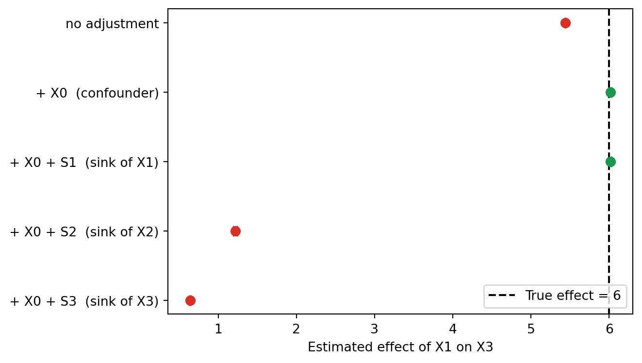

Figure 2: Posterior estimate of the X1 → X3 effect under each adjustment choice, with 94% HDIs. Only adjusting for the confounder X0 (optionally plus the harmless sink S1) recovers the true effect of 6 (black dashed). The empty set is confounded; conditioning on the mediator’s sink S2 or the outcome’s sink S3 induces severe bias.

The pathmc-native estimate: do() on the full house

Fitting X3 ~ b*X1 + X0 works, but it leans on the analyst to have already found the right adjustment set. The structural model removes that burden: once the full house is specified, ate() issues a do(X1) intervention and propagates it through the graph, automatically severing the backdoor through X0 without us naming a single covariate.

house.fit(draws=500, tune=500, chains=2, random_seed=42, progressbar=False)

ate = house.ate("X3", "X1", values=(0.0, 1.0))
print(f"True effect: {TRUE_EFFECT}")
ate

NUTS[nutpie]: [sigma_X3, beta_X3, sigma_X2, sigma_X1, beta_X1, beta_X2, beta_S3, beta_S2, beta_S1, sigma_S3, sigma_S2, sigma_S1]

True effect: 6.0

ATE of X1 on X3

Mean	6.00
94% HDI	[6.00, 6.01]
P(> 0)	1.00
Draws	1000

Methods: .hdi() .prob() .summary() .draws() .by_time() .dataset

The interventional estimate recovers the true effect of 6 directly from the DAG — no adjustment set to choose, no sink to accidentally include.

A sanity check on the DAG itself

adjustment_sets() reasons about the structure you declared; it cannot know whether that structure matches reality. test_implications() closes the loop by testing every conditional independence the house implies against the observed data.

house.test_implications()

DAG Implication Tests (α = 0.05)

✗ 5 of 14 implied independences violated.

Independence	Partial r	p-value	Pass
S1 ⊥⊥ S2 \| {X1, X2}	-0.007	0.0230	✗
S1 ⊥⊥ S3 \| {X1, X3}	-0.000	0.9374	✓
S1 ⊥⊥ X0 \| {X1}	0.003	0.3287	✓
S1 ⊥⊥ X2 \| {X1}	-0.001	0.6742	✓
S1 ⊥⊥ X3 \| {X0, X1, X2}	0.003	0.3128	✓
S2 ⊥⊥ S3 \| {X2, X3}	0.003	0.4012	✓
S2 ⊥⊥ X0 \| {X2}	-0.000	0.9945	✓
S2 ⊥⊥ X1 \| {X0, X2}	0.008	0.0147	✗
S2 ⊥⊥ X3 \| {X0, X2}	-0.001	0.6488	✓
S3 ⊥⊥ X0 \| {X3}	-0.008	0.0101	✗
S3 ⊥⊥ X1 \| {X0, X3}	-0.001	0.6507	✓
S3 ⊥⊥ X2 \| {X1, X3}	-0.008	0.0133	✗
X0 ⊥⊥ X2 \| {X1}	-0.007	0.0281	✗
X1 ⊥⊥ X3 \| {X0, X2}	0.000	0.9645	✓

The house implies fourteen conditional independences, and every partial correlation comes back negligible (|r| < 0.05) — consistent with a correctly specified DAG, which is unsurprising since we simulated directly from it. At this sample size the test is powerful enough that, across many simultaneous comparisons, one may land just under the α = 0.05 threshold despite an essentially zero correlation; that is a multiple-testing artefact, not evidence of a missing edge. The adjustment verdict above rests on a structure the data do not contradict.

Summary

Node	Verdict	Why
`X0`	Must adjust	Confounder; blocks the backdoor `X1 ← X0 → X3`. The only member of the unique valid set `{X0}`.
`S1`	Can adjust (optional)	Childless descendant of `X1` on no `X1`–`X3` path; harmless but unnecessary.
`X2`	Must avoid	Mediator; conditioning severs the causal path `X1 → X2 → X3`.
`S2`	Must avoid	Proxy for the mediator `X2`; partially blocks the causal path.
`S3`	Must avoid	Descendant of the outcome `X3`; conditioning bleeds away outcome variation.

adjustment_sets() answers the puzzle in one call: the unique minimal valid set is {X0}, which simultaneously says “adjust for X0” and “never condition on the descendants X2, S1, S2, S3.”
The backdoor criterion’s “no descendants of the treatment” rule disqualifies every S node and the mediator at once — including S2 and S3, whose bias is not collider bias and so is invisible to collider_warnings().
Fitting confirms the structure: adjusting for X0 (with or without the harmless S1) recovers the true effect of 6, while conditioning on S2 or S3 drives the estimate far from the truth.
do() on the full structural model recovers the effect with no manual adjustment-set selection at all — the graph does the work.

Try it yourself

Swap X3 ~ b*X1 + X0 + S2 for X3 ~ b*X1 + X0 + X2 and refit. Conditioning on the mediator X2 directly (rather than its noisy sink S2) drives the X1 coefficient essentially to zero — the cleanest demonstration that mediators must stay out of a total-effect adjustment set.