Vaccine Efficacy and Surrogate Endpoints
Assess whether a biomarker is a valid surrogate endpoint for clinical outcomes using mediation analysis.
Vaccine trials are expensive and slow. A Phase III efficacy trial might require tens of thousands of participants followed for months to observe enough clinical events (hospitalizations, severe disease) to establish that the vaccine works. If a biomarker measured early — such as antibody levels after vaccination — could reliably predict the clinical outcome, regulators could approve vaccines faster using the biomarker as a surrogate endpoint.
But when is a surrogate valid? The answer depends on the causal structure linking the vaccine, the biomarker, and the clinical outcome. If the vaccine works entirely through antibodies, then antibody levels are a perfect surrogate. But if the vaccine also confers protection through other mechanisms (T-cell immunity, mucosal defenses), antibody levels alone understate the true efficacy — and a surrogate-only trial could reject an effective vaccine.
This is a mediation question, and path analysis provides a principled framework for answering it.
The causal structure
The key quantities are:
| Effect | Meaning | Why it matters |
|---|---|---|
| Total (a × b + c) | Full causal effect of vaccination on hospitalization | The quantity regulators care about |
| Indirect (a × b) | Effect mediated through antibodies | What a surrogate-only trial captures |
| Direct (c) | Effect through non-antibody mechanisms | What a surrogate-only trial misses |
| Proportion mediated | Indirect / Total | How “valid” the surrogate is |
ImportantThe nonlinearity problem
In linear-Gaussian models, the indirect effect is simply the product of path coefficients: a × b. But when the outcome is binary (hospitalized: yes/no), the coefficients live on the log-odds scale, and the product a × b does not have a clean interpretation on the probability scale.
The do() operator handles this correctly: it propagates interventions through the full DAG, applying the inverse-logit transform at the Bernoulli stage, giving effects on the probability scale — the scale that matters for clinical decisions.
Simulate an observational cohort
We simulate an observational study of 1000 patients, where vaccination status is partially confounded by age (older patients are slightly more likely to seek vaccination).
import numpy as np
import pandas as pd
import matplotlib.pyplot as plt
from scipy.special import expit
import arviz as az
import pymc as pm
import pathmc

FIG_WIDTH = 8
FIG_HEIGHT = 4
COLOR_VACCINE = "#2171b5"
COLOR_ANTIBODY = "#31a354"
COLOR_HOSPITALIZED = "#e6550d"
COLOR_DIRECT = "#756bb1"

rng = np.random.default_rng(42)
n = 1000

age = rng.normal(0, 1, size=n)
comorbidity = np.abs(rng.normal(0, 1, size=n))

p_vax = expit(0.1 + 0.2 * age)
vaccine = rng.binomial(1, p_vax).astype(float)

true_a = 2.5
true_b_logit = -0.4
true_c_logit = -0.5
true_age_antibody = -0.3
true_age_hosp = 0.4
true_comorbidity_hosp = 0.5

antibody = (
    3.0 + true_a * vaccine + true_age_antibody * age + rng.normal(scale=0.8, size=n)
)

logit_hosp = (
    -0.5
    + true_b_logit * antibody
    + true_c_logit * vaccine
    + true_age_hosp * age
    + true_comorbidity_hosp * comorbidity
)
p_hosp = expit(logit_hosp)
hospitalized = rng.binomial(1, p_hosp).astype(float)

df = pd.DataFrame({
    "vaccine": vaccine,
    "age": age,
    "comorbidity": comorbidity,
    "antibody": antibody,
    "hospitalized": hospitalized,
})

print(f"N = {n}")
print(f"Vaccination rate:      {vaccine.mean():.1%}")
print(f"Hospitalization rate:  {hospitalized.mean():.1%}")
print(f"  Vaccinated:          {hospitalized[vaccine == 1].mean():.1%}")
print(f"  Unvaccinated:        {hospitalized[vaccine == 0].mean():.1%}")
df.head()
N = 1000
Vaccination rate: 53.7%
Hospitalization rate: 12.0%
Vaccinated: 8.0%
Unvaccinated: 16.6%| vaccine | age | comorbidity | antibody | hospitalized | |
|---|---|---|---|---|---|
| 0 | 1.0 | 0.304717 | 0.059283 | 4.332930 | 0.0 |
| 1 | 0.0 | -1.039984 | 0.729287 | 2.684588 | 0.0 |
| 2 | 1.0 | 0.750451 | 0.414473 | 5.174829 | 0.0 |
| 3 | 1.0 | 0.940565 | 0.633910 | 4.729751 | 0.0 |
| 4 | 0.0 | -1.951035 | 0.002993 | 5.425042 | 0.0 |
The raw rate difference is a mix of the true causal effect and confounding by age. Older patients are both more likely to be vaccinated and more likely to be hospitalized, which attenuates the apparent vaccine efficacy.
Visualise the data
Code
fig, axes = plt.subplots(1, 2, figsize=(FIG_WIDTH, FIG_HEIGHT))

ax = axes[0]
for vax_val, color, label in [
    (0, COLOR_HOSPITALIZED, "Unvaccinated"),
    (1, COLOR_VACCINE, "Vaccinated"),
]:
    vals = antibody[vaccine == vax_val]
    x_kde, y_kde, _ = az.kde(vals)
    ax.plot(x_kde, y_kde, color=color, lw=2, label=label)
    ax.fill_between(x_kde, y_kde, alpha=0.3, color=color)
ax.set_xlabel("Antibody level")
ax.set_ylabel("Density")
ax.legend()

ax = axes[1]
hosp_by_vax = df.groupby("vaccine")["hospitalized"].mean()
bars = ax.bar(
    ["Unvaccinated", "Vaccinated"],
    [hosp_by_vax[0], hosp_by_vax[1]],
    color=[COLOR_HOSPITALIZED, COLOR_VACCINE],
    alpha=0.7,
)
ax.set_ylabel("Hospitalization rate")
ax.set_ylim(0, max(hosp_by_vax) * 1.3)
for bar, val in zip(bars, [hosp_by_vax[0], hosp_by_vax[1]]):
    ax.text(
        bar.get_x() + bar.get_width() / 2,
        bar.get_height() + 0.01,
        f"{val:.1%}",
        ha="center",
        fontsize=10,
    )

plt.tight_layout()
plt.show()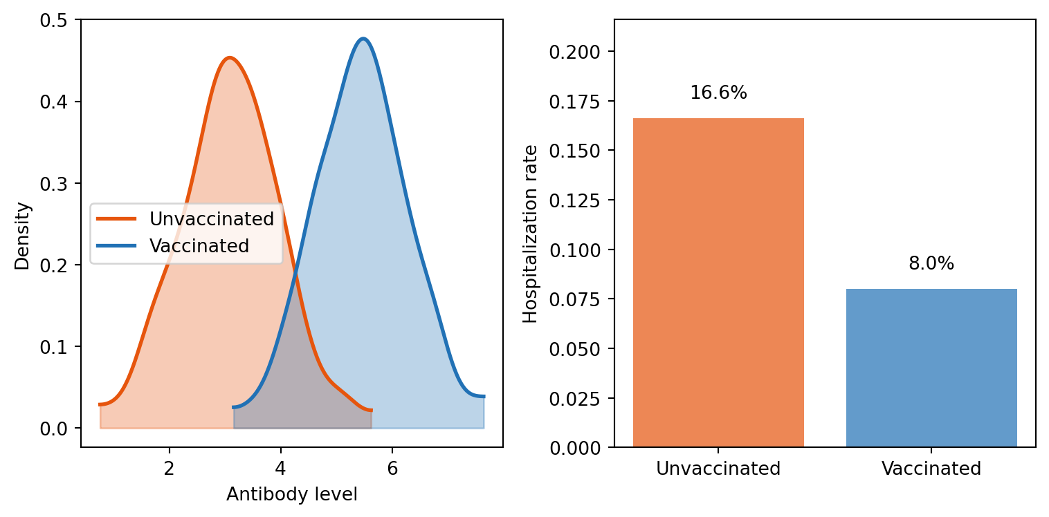
Code
fig, axes = plt.subplots(1, 2, figsize=(FIG_WIDTH, FIG_HEIGHT))

ax = axes[0]
age_bins = pd.qcut(age, 4, labels=["Young", "Mid-young", "Mid-old", "Old"])
hosp_by_age = df.assign(age_group=age_bins).groupby("age_group")["hospitalized"].mean()
ax.bar(hosp_by_age.index, hosp_by_age.values, color=COLOR_HOSPITALIZED, alpha=0.7)
ax.set_ylabel("Hospitalization rate")
ax.set_ylim(0, max(hosp_by_age) * 1.3)

ax = axes[1]
vax_by_age = df.assign(age_group=age_bins).groupby("age_group")["vaccine"].mean()
ax.bar(vax_by_age.index, vax_by_age.values, color=COLOR_VACCINE, alpha=0.7)
ax.set_ylabel("Vaccination rate")
ax.set_ylim(0, 1)

plt.tight_layout()
plt.show()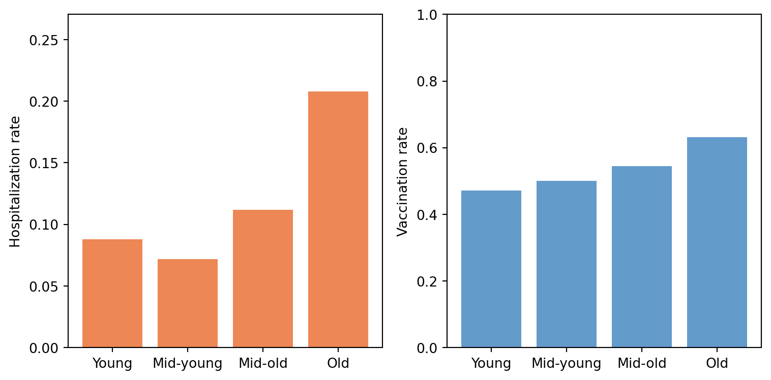
Specify and fit the path model
The spec encodes the full mediation structure. We use labeled coefficients for the three key paths (a, b, c) so we can inspect them separately.
spec = """
antibody     ~ a*vaccine + age
hospitalized ~ b*antibody + c*vaccine + age + comorbidity
"""

model = pathmc.model(
    spec,
    data=df,
    families={"hospitalized": "bernoulli"},
)
model.graph()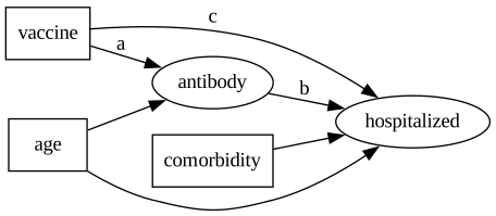
model.equations()\begin{aligned} \beta_{antibody} &\sim \text{Normal}(mu=0,\, sigma=10) \\ \sigma_{antibody} &\sim \text{HalfNormal}(sigma=1) \\ \beta_{hospitalized} &\sim \text{Normal}(mu=0,\, sigma=10) \\[6pt] \mu_{antibody} &= \beta_{0,\,antibody} + a \cdot \mathrm{vaccine} + \mathrm{age} \\ \mathrm{antibody} &\sim \text{Normal}(\mu_{antibody},\, \sigma_{antibody}) \\ \mu_{hospitalized} &= \beta_{0,\,hospitalized} \\ &\quad + b \cdot \mathrm{antibody} \\ &\quad + c \cdot \mathrm{vaccine} \\ &\quad + \mathrm{age} \\ &\quad + \mathrm{comorbidity} \\ \mathrm{hospitalized} &\sim \text{Bernoulli}(\text{logit}^{-1}(\mu_{hospitalized})) \end{aligned}
PyMC model graph
pm.model_to_graphviz(model.pymc_model)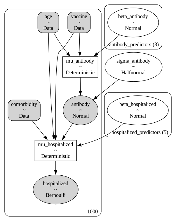
Sample
idata = model.fit(draws=1000, tune=1000, chains=4, random_seed=42)NUTS[nutpie]: [beta_hospitalized, sigma_antibody, beta_antibody]Results
Coefficient recovery
model.summary()| mean | sd | eti89_lb | eti89_ub | ess_bulk | ess_tail | r_hat | mcse_mean | mcse_sd | |
|---|---|---|---|---|---|---|---|---|---|
| beta_hospitalized[Intercept] | -0.997574 | 0.415363 | -1.642889 | -0.349081 | 947.620523 | 1196.563413 | 1.004304 | 0.013601 | 0.010033 |
| beta_hospitalized[antibody] | -0.448998 | 0.130704 | -0.654634 | -0.244290 | 881.600799 | 1076.378584 | 1.003982 | 0.004425 | 0.003296 |
| beta_hospitalized[vaccine] | -0.010825 | 0.387440 | -0.634046 | 0.595691 | 1129.865108 | 1508.926176 | 1.001924 | 0.011561 | 0.008451 |
| beta_hospitalized[age] | 0.452875 | 0.119994 | 0.258244 | 0.643366 | 3112.035274 | 3050.324710 | 1.003870 | 0.002154 | 0.001499 |
| beta_hospitalized[comorbidity] | 0.802241 | 0.156506 | 0.557713 | 1.054961 | 2485.583059 | 2694.736066 | 0.999758 | 0.003140 | 0.002189 |
| ... | ... | ... | ... | ... | ... | ... | ... | ... | ... |
| mu_antibody[995] | 5.361728 | 0.035119 | 5.306689 | 5.418633 | 5881.048440 | 3282.309657 | 1.000278 | 0.000458 | 0.000350 |
| mu_antibody[996] | 2.825315 | 0.044020 | 2.753675 | 2.894424 | 2686.326395 | 2387.966216 | 1.000432 | 0.000850 | 0.000575 |
| mu_antibody[997] | 3.019478 | 0.038272 | 2.957873 | 3.081356 | 2486.358837 | 2467.859306 | 1.000833 | 0.000767 | 0.000525 |
| mu_antibody[998] | 5.428476 | 0.034520 | 5.374515 | 5.484127 | 5895.181446 | 3296.013308 | 1.001211 | 0.000449 | 0.000343 |
| mu_antibody[999] | 2.808195 | 0.044765 | 2.734993 | 2.878510 | 2716.524592 | 2408.997958 | 1.000400 | 0.000860 | 0.000582 |
2009 rows × 9 columns
model.effects_summary()| mean | sd | hdi_3% | hdi_97% | |
|---|---|---|---|---|
| name | ||||
| a | 2.411880 | 0.051417 | 2.316049 | 2.509728 |
| b | -0.448998 | 0.130704 | -0.689899 | -0.214502 |
| c | -0.010825 | 0.387440 | -0.730935 | 0.703451 |
TipInterpreting the coefficients
- a (vaccine → antibody): on the identity scale. Vaccination increases antibody levels by ≈ 2.5 units. This is large and precisely estimated.
- b (antibody → hospitalized): on the log-odds scale. Each unit increase in antibody level decreases the log-odds of hospitalization by ≈ 0.4. The protective effect of antibodies.
- c (vaccine → hospitalized, direct): on the log-odds scale. The direct protective effect beyond what antibodies capture — other immune mechanisms.
Identification check
print(
    f"Is vaccine → hospitalized identifiable? {model.is_identifiable('vaccine', 'hospitalized')}"
)
print(f"Adjustment sets: {model.adjustment_sets('vaccine', 'hospitalized')}")
Is vaccine → hospitalized identifiable? True
Adjustment sets: [set()]Age must be in the adjustment set because it confounds both vaccine-antibody and vaccine-hospitalization relationships.
Causal effects on the probability scale
The coefficients above are on different scales (identity for antibody, log-odds for hospitalization). To get the quantities that matter for clinical decision-making, we use do() to compute effects on the probability scale.
Total vaccine efficacy
ate_vaccine = model.ate("hospitalized", "vaccine", values=(0.0, 1.0))
ate_vaccine
ATE of vaccine on hospitalized
| Mean | -0.10 |
| 94% HDI | [-0.14, -0.06] |
| P(> 0) | 0.00 |
| Draws | 4000 |
The negative value means vaccination reduces hospitalization probability — exactly what we’d hope.
Effect on the surrogate
The vaccine’s effect on antibody levels is on the identity scale, so we can also read it directly.
r_unvax = model.do(set={"vaccine": 0.0}, kind="mean")
r_vax = model.do(set={"vaccine": 1.0}, kind="mean")

print(f"E[antibody | do(vaccine=0)]: {r_unvax.mean('antibody'):.2f}")
print(f"E[antibody | do(vaccine=1)]: {r_vax.mean('antibody'):.2f}")
print(
    f"Antibody lift from vaccination: {r_vax.mean('antibody') - r_unvax.mean('antibody'):.2f}"
)
E[antibody | do(vaccine=0)]: 3.06
E[antibody | do(vaccine=1)]: 5.48
Antibody lift from vaccination: 2.41Decomposing the vaccine effect: is the surrogate sufficient?
This is the central question. If the vaccine’s entire effect flows through antibodies, then antibody levels are a sufficient surrogate — a trial measuring only antibodies could fully predict the clinical benefit.
We decompose the total effect into the indirect (through antibodies) and direct (non-antibody mechanisms) components using the controlled direct effect approach.
Total effect
Intervene on vaccination only, let antibody levels respond naturally:
r_total_0 = model.do(set={"vaccine": 0.0}, kind="mean")
r_total_1 = model.do(set={"vaccine": 1.0}, kind="mean")

total_effect = r_total_1 - r_total_0
print(f"Total effect on P(hospitalized): {total_effect.mean('hospitalized'):.4f}")
Total effect on P(hospitalized): -0.1030Controlled direct effect
To isolate the direct (non-antibody) mechanism, we intervene on both vaccine status and antibody level. By fixing antibody at its population mean, we block the indirect path — any remaining effect must be through the direct path.
mean_antibody = float(df["antibody"].mean())

r_cde_0 = model.do(set={"vaccine": 0.0, "antibody": mean_antibody}, kind="mean")
r_cde_1 = model.do(set={"vaccine": 1.0, "antibody": mean_antibody}, kind="mean")

controlled_direct = r_cde_1 - r_cde_0
print(
    f"Controlled direct effect on P(hospitalized): {controlled_direct.mean('hospitalized'):.4f}"
)
Controlled direct effect on P(hospitalized): -0.0014Indirect effect (through antibodies)
The indirect effect is the difference between the total and direct effects:
indirect_draws = total_effect.draws("hospitalized") - controlled_direct.draws(
    "hospitalized"
)

print(f"Indirect effect (via antibodies): {indirect_draws.mean():.4f}")

total_draws = total_effect.draws("hospitalized")
with np.errstate(divide="ignore", invalid="ignore"):
    prop_mediated = indirect_draws / total_draws
    prop_mediated = prop_mediated[np.isfinite(prop_mediated)]

print(f"Proportion mediated:             {np.mean(prop_mediated):.2f}")
Indirect effect (via antibodies): -0.1016
Proportion mediated: 1.03Code
fig, ax = plt.subplots(figsize=(FIG_WIDTH, FIG_HEIGHT))

for draws, color, label in [
    (total_effect.draws("hospitalized"), COLOR_VACCINE, "Total (all mechanisms)"),
    (indirect_draws, COLOR_ANTIBODY, "Indirect (via antibodies)"),
    (controlled_direct.draws("hospitalized"), COLOR_DIRECT, "Direct (non-antibody)"),
]:
    x_kde, y_kde, _ = az.kde(draws)
    ax.plot(x_kde, y_kde, color=color, lw=2, label=label)
    ax.fill_between(x_kde, y_kde, alpha=0.25, color=color)
    ax.axvline(draws.mean(), color=color, ls="--", alpha=0.7, lw=1)

ax.axvline(0, color="black", ls=":", alpha=0.3)
ax.set_xlabel("ΔP(hospitalized) from vaccination")
ax.set_ylabel("Density")
ax.legend()
plt.tight_layout()
plt.show()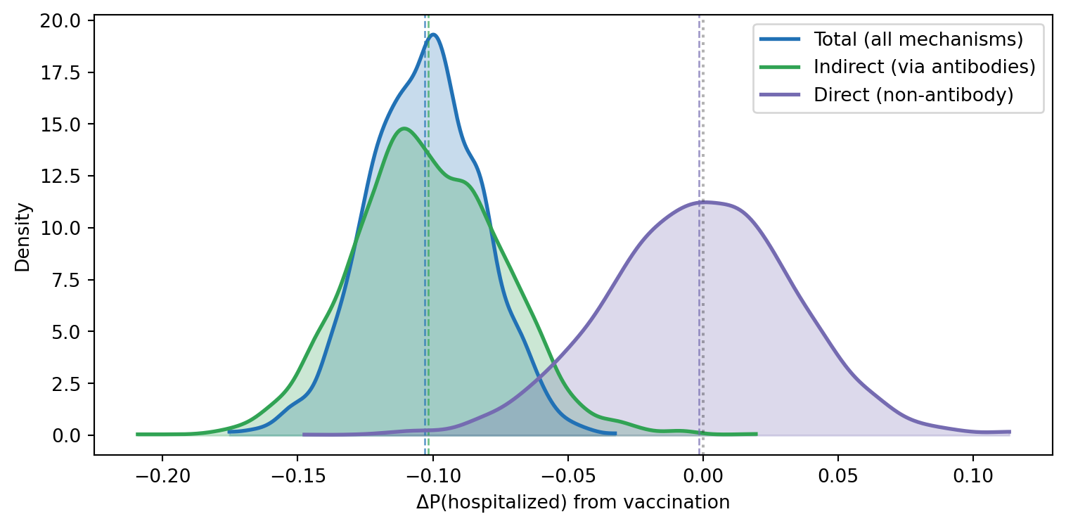
WarningSurrogate validity depends on the DAG
The proportion mediated tells us how much of the vaccine’s effect a surrogate-only trial would capture. In this simulation, antibodies mediate a large share of the total effect — substantial, but not everything.
A regulator relying only on antibody levels would underestimate the vaccine’s true efficacy by missing the direct protective mechanisms. Conversely, if a new vaccine variant has lower antibody response but preserves T-cell immunity, a surrogate-only trial might reject it even though it is clinically effective.
Confounding sensitivity
The causal estimates above assume all confounders are measured. What if there’s an unmeasured common cause of antibody levels and hospitalization — say, genetic factors affecting both immune response and disease severity?
We can’t test this from data, but we can check how sensitive our estimates are to the adjustment set.
warnings = model.collider_warnings({"age", "comorbidity"}, "vaccine", "hospitalized")
if warnings:
    for w in warnings:
        print(w)
else:
    print("No collider warnings for the current adjustment set.")
No collider warnings for the current adjustment set.Standardized effects
To compare effect magnitudes across predictors on different scales:
model.standardized()| predictor | outcome | mean | sd | hdi_3% | hdi_97% | |
|---|---|---|---|---|---|---|
| name | ||||||
| a | vaccine | antibody | 0.836226 | 0.017827 | 0.803000 | 0.870151 |
| b | antibody | hospitalized | -1.987111 | 0.578450 | -3.053255 | -0.949312 |
| c | vaccine | hospitalized | -0.016610 | 0.594497 | -1.121564 | 1.079393 |
Conditional vaccine efficacy
Does the vaccine work equally well for everyone? The cate() method lets us check whether vaccine efficacy varies with patient characteristics.
cate_young = model.cate(
    "hospitalized", "vaccine", values=(0.0, 1.0), condition={"age": -1.0}
)
cate_old = model.cate(
    "hospitalized", "vaccine", values=(0.0, 1.0), condition={"age": 1.0}
)

print("Vaccine effect by age group:")
print(
    f"  Young (age = -1 SD): ΔP(hosp) = {cate_young.mean():.4f}"
    f"  HDI: {cate_young.hdi(prob=0.94)}"
)
print(
    f"  Old (age = +1 SD):   ΔP(hosp) = {cate_old.mean():.4f}"
    f"  HDI: {cate_old.hdi(prob=0.94)}"
)
Vaccine effect by age group:
Young (age = -1 SD): ΔP(hosp) = -0.0632 HDI: [-0.09184514 -0.03801032]
Old (age = +1 SD): ΔP(hosp) = -0.1471 HDI: [-0.20378098 -0.08437929]
NoteWhy CATE varies even in a linear model
Even though the structural equations have no interaction terms, the CATE differs by age because of the logistic link function. The same change in log-odds translates to a larger change in probability when the baseline probability is near 0.5 than when it is near 0 or 1. Older patients have higher baseline hospitalization risk, so the same log-odds reduction from vaccination translates to a larger absolute risk reduction.
This is a fundamental property of nonlinear models: the treatment effect on the probability scale depends on where you start, even when the treatment effect on the log-odds scale is constant.
Code
ages = np.array([-1.5, -1.0, -0.5, 0.0, 0.5, 1.0, 1.5])
cate_draws_list = []

for a in ages:
    cate = model.cate(
        "hospitalized", "vaccine", values=(0.0, 1.0), condition={"age": float(a)}
    )
    cate_draws_list.append(cate.draws())

cate_draws_2d = np.column_stack(cate_draws_list)

fig, ax = plt.subplots(figsize=(FIG_WIDTH, FIG_HEIGHT))
ax.plot(ages, cate_draws_2d.mean(axis=0), "o-", color=COLOR_VACCINE, lw=2, ms=6)
hdi_1 = az.hdi(cate_draws_2d, prob=0.94, axis=0)
ax.fill_between(ages, hdi_1[:, 0], hdi_1[:, 1], alpha=0.2, color=COLOR_VACCINE)
ax.axhline(0, color="black", ls=":", alpha=0.3)
ax.set_xlabel("Age (standardized)")
ax.set_ylabel("ΔP(hospitalized) from vaccination")
plt.tight_layout()
plt.show()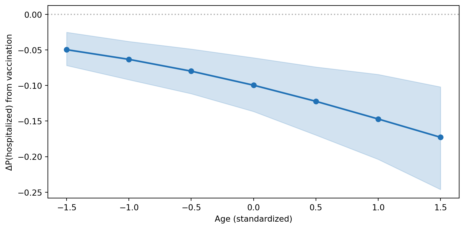
The vaccine is protective across all ages (all values are negative), but the absolute risk reduction is greatest for older, higher-risk patients.
Summary
- Surrogate endpoints are a mediation question. Whether a biomarker can substitute for a clinical endpoint depends on how much of the treatment’s effect flows through that biomarker — the proportion mediated.
- Mixed-family models handle continuous biomarkers (Gaussian) and binary clinical outcomes (Bernoulli) in the same DAG. do() applies the correct link function at each step.
- The controlled direct effect isolates the non-surrogate mechanism by intervening on both treatment and mediator. The indirect effect is the remainder: total minus direct.
- On the probability scale, effects are not additive. The logistic link means the same log-odds change produces different absolute risk changes depending on baseline risk. do() handles this automatically; manual coefficient arithmetic does not.
- Confounding by age attenuates the raw vaccine-outcome association. The path model adjusts for age in both equations, recovering the true causal effects.
- CATE reveals effect heterogeneity. Even without interaction terms, the vaccine’s absolute risk reduction varies by age due to the nonlinear link — a clinically important finding invisible to log-odds coefficients alone.
NoteReflection
In your own domain, which intermediate measurements might serve as surrogates for harder-to-measure outcomes?
- In clinical trials: is tumor shrinkage a valid surrogate for overall survival? What non-shrinkage mechanisms might the treatment have?
- In education: are test scores a valid surrogate for long-term career outcomes? Does improving test scores cause better outcomes, or just correlate with them?
- In product development: is user engagement a valid surrogate for retention? If you artificially boost engagement (gamification), does retention follow?
The answer always depends on the causal structure — and the proportion of the effect that flows through the proposed surrogate.