The do() Operator

Contrast conditioning P(Y|X=x) with intervening P(Y|do(X=x)), then master the full do() API — ATE, CATE, ATT/ATU, contrast arithmetic, and predictive propagation.

Author

Benjamin Vincent

“People who carry lighters are more likely to get lung cancer.” Should we ban lighters?

Obviously not — the association between lighters and cancer is not causal. Smoking is the common cause: it drives both lighter-carrying and cancer risk. Seeing someone carry a lighter updates our beliefs about their cancer risk (because we infer they probably smoke), but doing — forcibly giving someone a lighter — would not change their cancer risk at all.

This distinction between conditioning and intervening is the foundation of causal inference (Pearl et al. 2016, secs. 3.1–3.2). In notation: P(Y \mid X = x) tells us what we observe among units with a particular X value, while P(Y \mid do(X = x)) tells us what would happen if we set X by intervention, severing all non-causal paths into X.

pathmc makes the distinction concrete: filter the data to see what happens when X = x, or use do(X = x) to simulate an intervention. When confounding is present, the two give different answers — and only do() answers the causal question.

This notebook first builds intuition for why the distinction matters, then walks through pathmc’s full interventional API.

The confounded model

A confounder Z causes both X and Y. The true causal effect of X on Y is 0.4, but the observed association is larger because Z contributes through both paths.

Figure 1: Confounded fork: Z causes both X and Y. The observed X–Y association mixes the causal effect (X → Y) with spurious correlation through Z.

import numpy as np
import pandas as pd
import matplotlib.pyplot as plt
import pathmc

rng = np.random.default_rng(42)
n = 1000

Z = rng.normal(size=n)
X = 0.7 * Z + rng.normal(scale=0.5, size=n)

TRUE_EFFECT = 0.4
Y = TRUE_EFFECT * X + 0.6 * Z + rng.normal(scale=0.5, size=n)

df = pd.DataFrame({"X": X, "Y": Y, "Z": Z})

Seeing vs doing in the raw data

Before fitting any models, we can see the confounding directly. Figure 2 shows that the slope of Y on X in the raw data (the “seeing” slope) is steeper than the true causal effect. High-X individuals tend to have high Z, which independently raises Y — inflating the apparent relationship.

Code

FIG_WIDTH = 7
FIG_HEIGHT = 4

from numpy.polynomial.polynomial import polyfit

fig, ax = plt.subplots(figsize=(FIG_WIDTH, FIG_HEIGHT))

scatter = ax.scatter(X, Y, c=Z, cmap="viridis", alpha=0.4, s=15, rasterized=True)
cbar = plt.colorbar(scatter, ax=ax, label="Confounder Z")

raw_coeffs = polyfit(X, Y, 1)
x_range = np.linspace(X.min(), X.max(), 100)
ax.plot(
    x_range,
    raw_coeffs[0] + raw_coeffs[1] * x_range,
    "--",
    color="gray",
    linewidth=2,
    label=f"Raw slope = {raw_coeffs[1]:.2f} (seeing)",
)
ax.plot(
    x_range,
    np.mean(Y) + TRUE_EFFECT * (x_range - np.mean(X)),
    "--",
    color="black",
    linewidth=2,
    label=f"True causal slope = {TRUE_EFFECT} (doing)",
)

ax.set_xlabel("X")
ax.set_ylabel("Y")
ax.legend(loc="upper left", fontsize=9)
plt.tight_layout()
plt.show()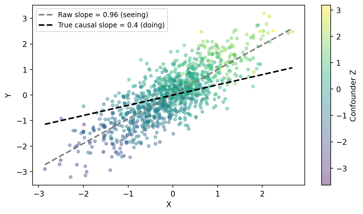

Figure 2: Scatter of X vs Y colored by the confounder Z. The raw regression slope (gray dashed) is steeper than the true causal effect (black dashed) because high-Z observations (yellow) push both X and Y upward simultaneously.

The gap between the gray and black lines is confounding bias. The raw slope picks up both X → Y and the spurious X ← Z → Y path. To recover the causal effect, we need to either adjust for Z or use do().

Seeing: P(Y | X = x)

To estimate what we see at a particular value of X, we take a narrow window of observations where X is close to a target value — approximating the conditional expectation E[Y \mid X = x]. This is purely observational: no model, no adjustment, just the data filtered to units whose X happens to fall near the target.

WINDOW = 0.2

lo_mask = (df["X"] > 0.0 - WINDOW) & (df["X"] < 0.0 + WINDOW)
hi_mask = (df["X"] > 1.0 - WINDOW) & (df["X"] < 1.0 + WINDOW)

y_see_lo = df.loc[lo_mask, "Y"].mean()
y_see_hi = df.loc[hi_mask, "Y"].mean()
z_see_lo = df.loc[lo_mask, "Z"].mean()
z_see_hi = df.loc[hi_mask, "Z"].mean()

print(
    f"E[Y | X ≈ 0] = {y_see_lo:.3f}   (n = {lo_mask.sum()},  mean Z in window = {z_see_lo:.2f})"
)
print(
    f"E[Y | X ≈ 1] = {y_see_hi:.3f}   (n = {hi_mask.sum()},  mean Z in window = {z_see_hi:.2f})"
)
print(f"Seeing difference:  {y_see_hi - y_see_lo:.3f}")
print(f"True causal effect: {TRUE_EFFECT}")

E[Y | X ≈ 0] = 0.066   (n = 198,  mean Z in window = 0.04)
E[Y | X ≈ 1] = 1.032   (n = 68,  mean Z in window = 1.06)
Seeing difference:  0.965
True causal effect: 0.4

The seeing difference is far larger than the true causal effect of 0.4. The mean Z in window column reveals why: among observations where X \approx 1, the average Z is about 1.0 — far above the population mean. Because Z causes X (the arrow Z \to X in the DAG), selecting high-X observations also selects high-Z observations. And since Z directly raises Y, the conditional mean E[Y \mid X \approx 1] is inflated by the “extra” Z that comes bundled with high X values.

Doing: P(Y | do(X = x))

The do() operator performs graph surgery (Pearl 2009): it severs all arrows into X and forces it to a value. This simulates an experiment where we assign X, breaking the link between Z and X. The post-intervention DAG has no Z → X edge, so Z no longer confounds the estimate.

spec = """
X ~ Z
Y ~ X + Z
"""

model = pathmc.model(spec, data=df)
model.equations()

\begin{aligned} \beta_{X} &\sim \text{Normal}(mu=0,\, sigma=10) \\ \sigma_{X} &\sim \text{HalfNormal}(sigma=1) \\ \beta_{Y} &\sim \text{Normal}(mu=0,\, sigma=10) \\ \sigma_{Y} &\sim \text{HalfNormal}(sigma=1) \\[6pt] \mu_{X} &= \beta_{0,\,X} + \mathrm{Z} \\ \mathrm{X} &\sim \text{Normal}(\mu_{X},\, \sigma_{X}) \\ \mu_{Y} &= \beta_{0,\,Y} + \mathrm{X} + \mathrm{Z} \\ \mathrm{Y} &\sim \text{Normal}(\mu_{Y},\, \sigma_{Y}) \end{aligned}

model.fit(draws=500, tune=500, chains=4, random_seed=42)

NUTS[nutpie]: [beta_Y, sigma_X, beta_X, sigma_Y]

r_do_lo = model.do(set={"X": 0.0})
r_do_hi = model.do(set={"X": 1.0})

causal_contrast = r_do_hi - r_do_lo
causal_contrast

DoResult — 2000 draws, 3 variables

variable	mean	94% HDI
Z	0.00	[0.00, 0.00]
X	1.00	[1.00, 1.00]
Y	0.38	[0.31, 0.44]

Methods: .draws() .mean() .hdi() .by_time() .dataset

The do() contrast uses the same 0-to-1 comparison as the seeing calculation above, but now the estimate lands on the true causal effect (TRUE_EFFECT = 0.4). Graph surgery breaks the Z \to X link, so high X no longer implies high Z — the confounding path is severed.

Side by side: seeing ≠ doing

The .ate() method wraps the entire do-calculus pipeline into a single call: specify the outcome, the treatment, and two contrast values, and pathmc returns an EstimandResult — a full posterior over the causal effect that already knows its outcome variable.

ate = model.ate("Y", "X", values=(0.0, 1.0))
ate

ATE of X on Y

Mean	0.38
94% HDI	[0.31, 0.44]
P(> 0)	1.00
Draws	2000

Methods: .hdi() .prob() .summary() .draws() .by_time() .dataset

The result table shows the posterior mean, HDI, P(> 0), and draw count — no separate accessor calls needed.

Code

fig, ax = plt.subplots(figsize=(FIG_WIDTH, FIG_HEIGHT * 0.65))

causal_val = ate.mean()
causal_hdi = ate.hdi(prob=0.94)
seeing_diff = y_see_hi - y_see_lo

ax.errorbar(
    seeing_diff,
    1,
    fmt="s",
    color="C3",
    markersize=8,
    label="Seeing (conditional difference)",
)
ax.errorbar(
    causal_val,
    0,
    xerr=[[causal_val - causal_hdi[0]], [causal_hdi[1] - causal_val]],
    fmt="o",
    color="C0",
    capsize=5,
    label="Doing (do-operator ATE)",
)
ax.axvline(
    TRUE_EFFECT,
    color="black",
    linestyle="--",
    label=f"True causal effect ({TRUE_EFFECT})",
)
ax.set_yticks([0, 1])
ax.set_yticklabels(["do(X=1) − do(X=0)", "E[Y|X≈1] − E[Y|X≈0]"])
ax.set_xlabel("Effect of X on Y")
ax.legend(loc="best", fontsize=9)
plt.tight_layout()
plt.show()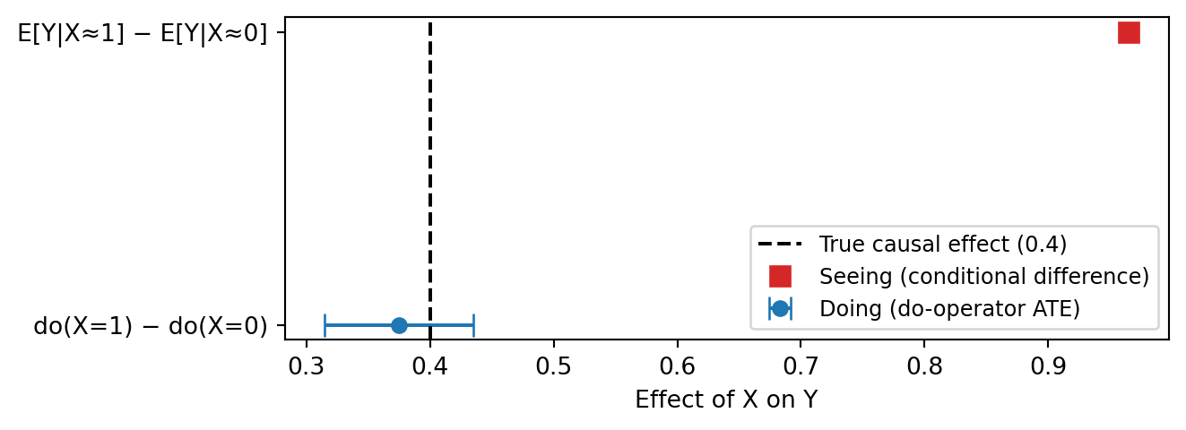

Figure 3: Under confounding, the conditional difference (seeing) overestimates the causal effect by more than 2×. The do-operator recovers the true effect of 0.4. Black dashed line marks the true DGP value.

When seeing = doing: no confounding

If X is randomized (no common cause with Y), there is no confounding and the observational association equals the causal effect. The do() operator becomes redundant — but it doesn’t hurt. This is the experimental ideal: random assignment makes the association causal by design.

X_rand = rng.normal(size=n)
Y_rand = TRUE_EFFECT * X_rand + rng.normal(scale=0.5, size=n)

df_rand = pd.DataFrame({"X": X_rand, "Y": Y_rand})

model_rand = pathmc.model("Y ~ X", data=df_rand)
model_rand.fit(draws=500, tune=500, chains=4, random_seed=42)

NUTS[nutpie]: [beta_Y, sigma_Y]

Without confounding, the regression slope of Y on X — the “seeing” estimate — should match the do-operator ATE. Both should recover the true causal effect.

seeing_slope = polyfit(X_rand, Y_rand, 1)[1]
print(f"Seeing  (OLS slope): {seeing_slope:.3f}   True effect: {TRUE_EFFECT}")

Seeing  (OLS slope): 0.402   True effect: 0.4

ate_rand = model_rand.ate("Y", "X", values=(0.0, 1.0))
ate_rand

ATE of X on Y

Mean	0.40
94% HDI	[0.37, 0.43]
P(> 0)	1.00
Draws	2000

Methods: .hdi() .prob() .summary() .draws() .by_time() .dataset

Code

fig, ax = plt.subplots(figsize=(FIG_WIDTH, FIG_HEIGHT * 0.65))

rand_val = ate_rand.mean()
rand_hdi = ate_rand.hdi(prob=0.94)

ax.errorbar(
    seeing_slope,
    1,
    fmt="s",
    color="C1",
    markersize=8,
    label="Seeing (OLS slope)",
)
ax.errorbar(
    rand_val,
    0,
    xerr=[[rand_val - rand_hdi[0]], [rand_hdi[1] - rand_val]],
    fmt="o",
    color="C0",
    capsize=5,
    label="Doing (do-operator ATE)",
)
ax.axvline(
    TRUE_EFFECT,
    color="black",
    linestyle="--",
    label=f"True causal effect ({TRUE_EFFECT})",
)
ax.set_yticks([0, 1])
ax.set_yticklabels(["do(X=1) − do(X=0)", "OLS slope"])
ax.set_xlabel("Effect of X on Y")
ax.legend(loc="best", fontsize=9)
plt.tight_layout()
plt.show()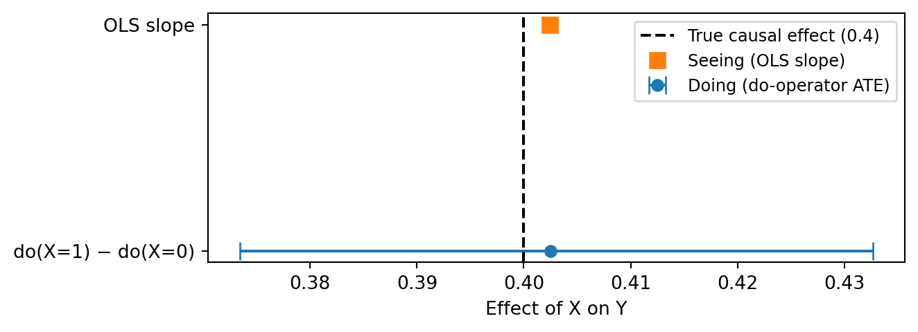

Figure 4: Without confounding (randomized X), the OLS slope and the do-operator agree — both recover the true causal effect of 0.4.

We’ve established why do() matters. Now let’s explore the full API — how to ask different causal questions using the same fitted model.

The do() API

Average treatment effect

The ATE compares two interventions: setting X = 1 versus X = 0. The .ate() method is shorthand for the two-do() contrast:

ate = model.ate("Y", "X", values=(0.0, 1.0))
ate

ATE of X on Y

Mean	0.38
94% HDI	[0.31, 0.44]
P(> 0)	1.00
Draws	2000

Methods: .hdi() .prob() .summary() .draws() .by_time() .dataset

The EstimandResult also answers decision-oriented questions directly. float() collapses it to the posterior mean, .prob() reports the posterior probability that the effect clears a threshold, and .summary() returns a tidy one-row table:

print(f"Posterior mean:  {float(ate):.3f}")
print(f"P(ATE > 0):      {ate.prob('> 0'):.3f}")
ate.summary()

Posterior mean:  0.375
P(ATE > 0):      1.000

	outcome	treatment	mean	sd	hdi_3%	hdi_97%	p(>0)
estimand
ATE	Y	X	0.375083	0.03204	0.314983	0.435037	1.0

This is equivalent to the manual contrast with do(). The manual contrast returns a DoResult (no privileged outcome), so its accessors still take a variable name:

r0 = model.do(set={"X": 0.0})
r1 = model.do(set={"X": 1.0})
manual_ate = r1 - r0
print(f"Manual ATE:    {manual_ate.mean('Y'):.3f}")

Manual ATE:    0.375

Conditional average treatment effect

.cate() fixes additional variables at specific values in both scenarios. This answers: “what is the causal effect of X on Y when Z is held at a particular level?”

cate_z_low = model.cate("Y", "X", values=(0.0, 1.0), condition={"Z": -1.0})
cate_z_high = model.cate("Y", "X", values=(0.0, 1.0), condition={"Z": 2.0})

print(f"CATE at Z = -1: {cate_z_low.mean():.3f}")
print(f"CATE at Z =  2: {cate_z_high.mean():.3f}")
print(f"ATE (no cond):  {ate.mean():.3f}")

CATE at Z = -1: 0.375
CATE at Z =  2: 0.375
ATE (no cond):  0.375

In a linear model without interactions, the CATE equals the ATE regardless of the conditioning value — the X → Y coefficient does not depend on Z. The values match because Z’s contribution cancels out in the contrast.

When does CATE differ from ATE?

CATE becomes informative when the treatment effect varies with a moderator — for example, in models with interaction terms or nonlinear specifications. In those cases, .cate() lets you examine how the causal effect changes across subgroups.

Contrast arithmetic

DoResult objects support subtraction, producing a new DoResult whose draws are the element-wise difference. This makes it easy to build arbitrary contrasts:

r_low = model.do(set={"X": -1.0})
r_high = model.do(set={"X": 2.0})

contrast = r_high - r_low
contrast

DoResult — 2000 draws, 3 variables

variable	mean	94% HDI
Z	0.00	[0.00, 0.00]
X	3.00	[3.00, 3.00]
Y	1.13	[0.94, 1.31]

Methods: .draws() .mean() .hdi() .by_time() .dataset

Since the model is linear, the effect should scale proportionally: a shift of 3 units in X should produce roughly 3 × 0.4 = 1.2 units of change in Y.

Inspecting individual do() results

Each DoResult holds the posterior-predictive distribution for every variable under the intervention:

scenario = model.do(set={"X": 1.0})

print(f"E[Y | do(X=1)]:  {scenario.mean('Y'):.3f}")
print(f"E[X | do(X=1)]:  {scenario.mean('X'):.3f}")

E[Y | do(X=1)]:  0.373
E[X | do(X=1)]:  1.000

Mean vs predictive propagation

By default, do() uses kind="mean", which propagates deterministically through the DAG — each variable is computed as the exact linear combination of its parents’ values and the posterior coefficient draws. This captures parameter uncertainty but not residual noise.

With kind="predictive", residual noise is added at each step: for Gaussian variables, a draw from Normal(0, sigma) using the posterior sigma; for Bernoulli variables, a binary draw from Bernoulli(p). The result is a full posterior predictive distribution that reflects both sources of uncertainty.

r_mean = model.do(set={"X": 1.0}, kind="mean")
r_pred = model.do(set={"X": 1.0}, kind="predictive")

hdi_mean = r_mean.hdi("Y")
hdi_pred = r_pred.hdi("Y")

print(
    f"Mean propagation  - 94% HDI: [{hdi_mean[0]:.3f}, {hdi_mean[1]:.3f}]  width={hdi_mean[1] - hdi_mean[0]:.3f}"
)
print(
    f"Predictive draws  - 94% HDI: [{hdi_pred[0]:.3f}, {hdi_pred[1]:.3f}]  width={hdi_pred[1] - hdi_pred[0]:.3f}"
)

Sampling: [Y]

Mean propagation  - 94% HDI: [0.307, 0.448]  width=0.140
Predictive draws  - 94% HDI: [-1.145, 1.901]  width=3.045

The predictive HDI is wider because it includes residual variation around the regression line. Use kind="mean" when you want to isolate the causal effect (parameter uncertainty only), and kind="predictive" when you want to predict the actual distribution of outcomes under an intervention.

Subgroup treatment effects: ATT and ATU

The ATE averages the treatment effect over the entire covariate distribution. But when effect modification is present — the treatment effect depends on a covariate — different subgroups experience different effects. The ATT (average treatment effect on the treated) and ATU (average treatment effect on the untreated) average over the covariate distributions of the treated and untreated subgroups respectively.

This section uses a binary treatment with confounding and effect modification to demonstrate when and why these estimands diverge.

seed = sum(map(ord, "att atu"))
rng_att = np.random.default_rng(seed=seed)
n_att = 500

truth = {
    "treatment_effect": 0.5,
    "confounder_effect": 0.3,
    "confounder_on_trt": 0.8,
    "interaction_effect": 0.4,
}

X_att = rng_att.normal(size=n_att)
prob_T = 1 / (1 + np.exp(-truth["confounder_on_trt"] * X_att))
T_att = (rng_att.uniform(size=n_att) < prob_T).astype(float)


def expected_y(T_val, X_val):
    return (
        truth["treatment_effect"] * T_val
        + truth["confounder_effect"] * X_val
        + truth["interaction_effect"] * T_val * X_val
    )


noise_att = rng_att.normal(scale=0.5, size=n_att)
Y_att = expected_y(T_att, X_att) + noise_att

df_att = pd.DataFrame({"X": X_att, "T": T_att, "Y": Y_att})

truth["true_ate"] = (expected_y(1, X_att) - expected_y(0, X_att)).mean()
truth["true_att"] = (
    expected_y(1, X_att[T_att == 1]) - expected_y(0, X_att[T_att == 1])
).mean()
truth["true_atu"] = (
    expected_y(1, X_att[T_att == 0]) - expected_y(0, X_att[T_att == 0])
).mean()

print(f"True ATE: {truth['true_ate']:.3f}")
print(f"True ATT: {truth['true_att']:.3f}")
print(f"True ATU: {truth['true_atu']:.3f}")
print(f"\nE[X | T=1] = {X_att[T_att == 1].mean():.2f}")
print(f"E[X | T=0] = {X_att[T_att == 0].mean():.2f}")

True ATE: 0.466
True ATT: 0.612
True ATU: 0.342

E[X | T=1] = 0.28
E[X | T=0] = -0.39

Because X positively affects both treatment probability and the treatment effect size (via the interaction), the treated subgroup has higher X on average, making ATT > ATE > ATU.

model_att = pathmc.model("Y ~ T + X + T:X", data=df_att)
model_att.fit(draws=500, tune=500, chains=4, random_seed=42)

NUTS[nutpie]: [beta_Y, sigma_Y]

ate_att = model_att.ate("Y", "T", values=(0.0, 1.0))
att = model_att.att("Y", "T", values=(0.0, 1.0), treated_value=1.0)
atu = model_att.atu("Y", "T", values=(0.0, 1.0), untreated_value=0.0)

print(f"{'Estimand':<12} {'Estimate':>10} {'True':>10}")
print(f"{'ATE':<12} {ate_att.mean():>10.3f} {truth['true_ate']:>10.3f}")
print(f"{'ATT':<12} {att.mean():>10.3f} {truth['true_att']:>10.3f}")
print(f"{'ATU':<12} {atu.mean():>10.3f} {truth['true_atu']:>10.3f}")

Estimand       Estimate       True
ATE               0.461      0.466
ATT               0.616      0.612
ATU               0.329      0.342

When to use ATT vs ATU vs ATE

ATT: “How much did the treatment help those who received it?” — useful for evaluating an existing policy or program.
ATU: “How much would the treatment help those who haven’t received it yet?” — useful for decisions about expanding a program.
ATE: “What is the average effect across the whole population?” — useful when the policy will be applied uniformly.

In a linear model without interactions, all three are equal. They diverge when the treatment effect is heterogeneous and treatment assignment is correlated with the source of heterogeneity.

When do() is not enough

do() assumes the DAG is correctly specified and all confounders are measured. If there is an unobserved common cause of X and Y that is not in the model, the do() result will still be biased — the method computes the mechanical consequence of the intervention under the given model, not ground truth.

Always pair do() with careful thinking about your causal assumptions. See Causal Identification for how to verify that your model identifies the effect you want, including what to do when confounders are unobserved.

Summary

Seeing is conditioning: P(Y \mid X = x). It reflects associations in the data, which can include confounding.
Doing is intervening: P(Y \mid do(X = x)). It simulates an experiment by severing all non-causal paths into X (Pearl et al. 2016, sec. 3.1).
When confounding is present, seeing ≠ doing. The scatter plot (Figure 2) makes this visible: the raw regression slope conflates causation and confounding.
When X is randomized (no confounders), seeing = doing. The association is the causal effect — this is why randomized experiments are the gold standard (Pearl and Mackenzie 2018, Ch. 4).
The do() API provides .ate(), .cate(), .att(), and .atu() for common causal queries — each returning an EstimandResult whose .mean(), .hdi(), and .prob() default to the outcome — plus raw do() and DoResult subtraction for custom contrasts.
Mean vs predictive propagation: kind="mean" isolates parameter uncertainty (for causal effects); kind="predictive" adds residual noise (for outcome prediction).
ATT and ATU diverge from ATE when effect modification is present and treatment assignment is correlated with the modifier.

Reflection

Think of an association in your domain that you suspect is confounded:

Advertising: Stores that advertise more have higher sales — but is that because advertising works, or because high-revenue stores have bigger budgets?
Education: Students who attend tutoring perform better on exams — but students who seek tutoring may already be more motivated.
Medicine: Patients who take a supplement report feeling better — but patients who buy supplements may also exercise more and eat better.

In each case, ask: “If I forced the treatment on a random person, would the outcome change?” That’s the do() question.

References

Pearl, Judea. 2009. Causality: Models, Reasoning, and Inference. 2nd ed. Cambridge University Press.

Pearl, Judea, Madelyn Glymour, and Nicholas P. Jewell. 2016. Causal Inference in Statistics: A Primer. John Wiley & Sons.

Pearl, Judea, and Dana Mackenzie. 2018. The Book of Why: The New Science of Cause and Effect. Basic Books.