Treatment Effects with Non-Linear Models

Why coefficients ≠ ATE in logistic models, AME vs MEM, g-computation for binary outcomes, and mixed-family models.

Author

Benjamin Vincent

When a treatment is binary and the model is linear, reading the causal effect is straightforward: the coefficient on treatment is the Average Treatment Effect. But this shortcut breaks when the outcome is binary and the model uses a logistic link. The same coefficient value means completely different things on the two scales.

This notebook demonstrates the difference with simulated data, verifies that pathmc’s do() operator correctly recovers the ATE in both cases, and explains why g-computation is the general solution. It closes with mixed-family models where continuous and binary variables coexist in the same DAG.

Setup

import numpy as np
import pandas as pd
import matplotlib.pyplot as plt
from scipy.special import expit
import arviz as az
import pathmc

FIG_WIDTH = 7
FIG_HEIGHT = 4
COLOR_LINEAR = "#2171b5"
COLOR_LOGISTIC = "#e6550d"
COLOR_TRUE = "#333333"

rng = np.random.default_rng(42)
n = 1000

The causal structure

Both models share the same DAG: a randomized binary treatment T and a pre-treatment covariate Z jointly affect the outcome Y. Because T is randomized (independent of Z), there is no confounding — we can focus purely on the link function.

Figure 1: Treatment T is randomized (no arrow from Z to T). Z is a pre-treatment covariate that affects Y.

The difference between the two models is the link function connecting the linear predictor to the outcome:

Linear: Y = \beta_0 + \beta_T T + \beta_Z Z + \varepsilon (identity link)
Logistic: P(Y{=}1) = \text{logit}^{-1}(\beta_0 + \beta_T T + \beta_Z Z) (logit link)

In both cases, the coefficient on T is exactly 1.0. The question is: does “coefficient = 1.0” mean the same thing for the causal effect?

Shared exogenous variables

Both models use the same covariate and treatment assignment:

Z = rng.normal(0, 1, size=n)
T = rng.binomial(1, 0.5, size=n).astype(float)

Linear model: ATE equals the coefficient

Simulate data

true_b0_lin = 2.0
true_bT_lin = 1.0
true_bZ_lin = 0.8

Y_linear = (
    true_b0_lin + true_bT_lin * T + true_bZ_lin * Z + rng.normal(scale=1.0, size=n)
)

df_linear = pd.DataFrame({"T": T, "Z": Z, "Y": Y_linear})
print(f"True coefficient on T: {true_bT_lin}")
print(f"True ATE:              {true_bT_lin}")

True coefficient on T: 1.0
True ATE:              1.0

In a linear model, the individual treatment effect is constant across all individuals:

\text{ITE}_i = (\beta_0 + \beta_T \cdot 1 + \beta_Z Z_i) - (\beta_0 + \beta_T \cdot 0 + \beta_Z Z_i) = \beta_T

The covariate terms cancel. The ATE is simply the coefficient, regardless of the distribution of Z.

Fit and verify

model_lin = pathmc.model("Y ~ bT*T + bZ*Z", data=df_linear)
model_lin.equations()

\begin{aligned} \beta_{Y} &\sim \text{Normal}(mu=0,\, sigma=10) \\ \sigma_{Y} &\sim \text{HalfNormal}(sigma=1) \\[6pt] \mu_{Y} &= \beta_{0,\,Y} + bT \cdot \mathrm{T} + bZ \cdot \mathrm{Z} \\ \mathrm{Y} &\sim \text{Normal}(\mu_{Y},\, \sigma_{Y}) \end{aligned}

model_lin.fit(draws=500, tune=500, chains=4, random_seed=42)

NUTS[nutpie]: [beta_Y, sigma_Y]

model_lin.effects_summary()

	mean	sd	hdi_3%	hdi_97%
name
bT	1.002885	0.066104	0.876797	1.124270
bZ	0.750636	0.032332	0.692716	0.813651

The coefficient bT is close to 1.0. Now let’s verify that do() agrees:

ate_lin = model_lin.ate("Y", "T", values=(0.0, 1.0))
ate_lin

ATE of T on Y

Mean	1.00
94% HDI	[0.88, 1.12]
P(> 0)	1.00
Draws	2000

Methods: .hdi() .prob() .summary() .draws() .by_time() .dataset

As expected, the result matches — for a linear model, the coefficient is the ATE.

Logistic model: ATE does NOT equal the coefficient

Simulate data

We use the same coefficient value (1.0) on the treatment, but now on the log-odds scale:

true_b0_log = -0.5
true_bT_log = 1.0
true_bZ_log = 1.5

logit_Y = true_b0_log + true_bT_log * T + true_bZ_log * Z
p_Y = expit(logit_Y)
Y_binary = rng.binomial(1, p_Y).astype(float)

df_logistic = pd.DataFrame({"T": T, "Z": Z, "Y": Y_binary})
print(f"P(Y=1) in data: {Y_binary.mean():.2f}")

P(Y=1) in data: 0.48

The true ATE on the probability scale

Unlike the linear case, the individual treatment effect depends on Z through the logistic transform:

\text{ITE}_i = \text{logit}^{-1}(\beta_0 + \beta_T + \beta_Z Z_i) - \text{logit}^{-1}(\beta_0 + \beta_Z Z_i)

The Z terms do not cancel because \text{logit}^{-1} is nonlinear. The ATE (risk difference) is the average of these individual effects over the population:

true_ite = expit(true_b0_log + true_bT_log + true_bZ_log * Z) - expit(
    true_b0_log + true_bZ_log * Z
)
true_ate_logistic = true_ite.mean()

print(f"Coefficient on T (log-odds):  {true_bT_log}")
print(f"Odds ratio exp(β_T):          {np.exp(true_bT_log):.2f}")
print(f"True ATE (risk difference):   {true_ate_logistic:.3f}")
print(f"ITE range:                    [{true_ite.min():.3f}, {true_ite.max():.3f}]")

Coefficient on T (log-odds):  1.0
Odds ratio exp(β_T):          2.72
True ATE (risk difference):   0.177
ITE range:                    [0.004, 0.245]

The coefficient is 1.0, the odds ratio is 2.72, and the ATE is ~0.19. Three numbers, three different scales, three different answers to “what is the treatment effect?”

Fit and verify

model_log = pathmc.model(
    "Y ~ bT*T + bZ*Z",
    data=df_logistic,
    families={"Y": "bernoulli"},
)
model_log.equations()

\begin{aligned} \beta_{Y} &\sim \text{Normal}(mu=0,\, sigma=10) \\[6pt] \mu_{Y} &= \beta_{0,\,Y} + bT \cdot \mathrm{T} + bZ \cdot \mathrm{Z} \\ \mathrm{Y} &\sim \text{Bernoulli}(\text{logit}^{-1}(\mu_{Y})) \end{aligned}

model_log.fit(draws=500, tune=500, chains=4, random_seed=42)

NUTS[nutpie]: [beta_Y]

model_log.effects_summary()

	mean	sd	hdi_3%	hdi_97%
name
bT	0.976511	0.149219	0.693851	1.24294
bZ	1.487962	0.106298	1.306464	1.69956

The coefficient bT is close to 1.0 — on the log-odds scale. This is NOT the ATE on the probability scale. To get the ATE (risk difference), we need do():

ate_log = model_log.ate("Y", "T", values=(0.0, 1.0))
ate_log

ATE of T on Y

Mean	0.17
94% HDI	[0.13, 0.22]
P(> 0)	1.00
Draws	2000

Methods: .hdi() .prob() .summary() .draws() .by_time() .dataset

The do() operator correctly computes the ATE on the probability scale — matching the true value (~0.19), not the coefficient of 1.0 on the log-odds scale.

What do() is doing: g-computation

pathmc’s do() implements g-computation (parametric standardization):

For each posterior draw of (\beta_0, \beta_T, \beta_Z):
Set T = 1 for every observation → predict P(Y{=}1 \mid T{=}1, Z_i)
Set T = 0 for every observation → predict P(Y{=}1 \mid T{=}0, Z_i)
Compute \text{ITE}_i for each observation
Average over observations → ATE for this posterior draw

The result is a full posterior distribution of the ATE, correctly accounting for both parameter uncertainty and the nonlinear link function.

Understanding the difference

The logistic curve

The core issue is the nonlinearity of the logistic function. In a linear model, a one-unit shift in the predictor always produces the same change in the outcome. In a logistic model, the same shift in log-odds produces different changes in probability depending on the baseline:

Code

x = np.linspace(-4, 4, 200)
y = expit(x)

fig, ax = plt.subplots(figsize=(FIG_WIDTH, FIG_HEIGHT))
ax.plot(x, y, color=COLOR_LOGISTIC, lw=2.5)

for start in [-3, -1, 1]:
    end = start + 1.0
    p_start = expit(start)
    p_end = expit(end)
    delta_p = p_end - p_start

    ax.annotate(
        "",
        xy=(end, p_start),
        xytext=(start, p_start),
        arrowprops=dict(arrowstyle="->", color=COLOR_TRUE, lw=1.5),
    )
    ax.annotate(
        "",
        xy=(end, p_end),
        xytext=(end, p_start),
        arrowprops=dict(arrowstyle="->", color=COLOR_LOGISTIC, lw=1.5),
    )
    ax.text(
        end + 0.15,
        (p_start + p_end) / 2,
        f"Δp = {delta_p:.2f}",
        fontsize=9,
        color=COLOR_LOGISTIC,
        va="center",
    )

ax.set_xlabel("Linear predictor (log-odds)")
ax.set_ylabel("P(Y = 1)")
plt.tight_layout()
plt.show()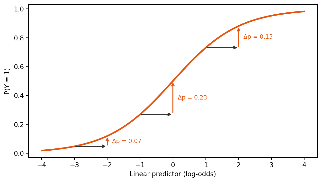

Figure 2: The logistic function. The same shift in log-odds (Δ = 1.0, horizontal arrows) produces different changes in probability (vertical arrows) depending on the baseline. Near the extremes, the effect is small; near the center, it is large.

Individual treatment effects

This nonlinearity means the treatment effect varies across individuals. In the linear model, every individual has the same ITE. In the logistic model, the ITE peaks where the baseline probability is near 0.5 and shrinks toward the extremes:

Code

z_grid = np.linspace(-3, 3, 200)
ite_linear = np.full_like(z_grid, true_bT_lin)
ite_logistic = expit(true_b0_log + true_bT_log + true_bZ_log * z_grid) - expit(
    true_b0_log + true_bZ_log * z_grid
)

fig, axes = plt.subplots(1, 2, figsize=(FIG_WIDTH, FIG_HEIGHT))

axes[0].plot(z_grid, ite_linear, color=COLOR_LINEAR, lw=2.5)
axes[0].axhline(true_bT_lin, color=COLOR_TRUE, ls="--", lw=1, alpha=0.5)
axes[0].set_xlabel("Z")
axes[0].set_ylabel("Individual treatment effect")
axes[0].set_title("Linear model")
axes[0].set_ylim(-0.05, 1.15)

axes[1].plot(z_grid, ite_logistic, color=COLOR_LOGISTIC, lw=2.5)
axes[1].axhline(
    true_ate_logistic,
    color=COLOR_TRUE,
    ls="--",
    lw=1,
    alpha=0.5,
    label=f"ATE = {true_ate_logistic:.3f}",
)
axes[1].set_xlabel("Z")
axes[1].set_title("Logistic model")
axes[1].set_ylim(-0.05, 0.30)
axes[1].legend()

plt.tight_layout()
plt.show()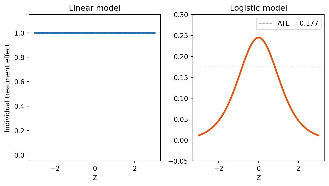

Figure 3: Individual treatment effects as a function of Z. Left: in the linear model, the ITE is constant (flat line at the coefficient value). Right: in the logistic model, the ITE varies with Z — individuals near the center of the probability scale benefit most.

The key insight

In a linear model, ATE = coefficient because subtracting two linear functions gives a constant — the covariate terms cancel.

In a logistic model, the ATE is the average of a nonlinear function of the covariates. It depends on the covariate distribution in the population and cannot be read from the coefficient alone. You need g-computation.

Marginal effect at the mean vs average marginal effect

A common shortcut for logistic models is to evaluate the treatment effect at the mean of the covariates — the marginal effect at the mean (MEM). This gives the ITE for a single “representative” individual, but it is not the ATE:

mem = expit(true_b0_log + true_bT_log + true_bZ_log * Z.mean()) - expit(
    true_b0_log + true_bZ_log * Z.mean()
)
ame = true_ate_logistic

print(f"Marginal effect at the mean (MEM):  {mem:.3f}")
print(f"Average marginal effect (AME/ATE):  {ame:.3f}")

Marginal effect at the mean (MEM):  0.245
Average marginal effect (AME/ATE):  0.177

The MEM overestimates the ATE because the logistic curve is concave near its center (Jensen’s inequality). pathmc’s do() computes the AME — the correct population-level ATE.

Which effect measure?

The logistic coefficient \beta_T gives rise to several legitimate effect measures, each answering a different question:

Measure	Formula	Interpretation
Log-odds ratio	\beta_T	Change in log-odds per unit treatment (constant)
Odds ratio	\exp(\beta_T)	Multiplicative change in odds (constant)
Risk difference (ATE)	E[\text{ITE}_i]	Average change in P(Y=1) (depends on covariates)
MEM	ITE at \bar{Z}	Treatment effect for a “typical” individual

The odds ratio is constant across individuals, which is why it’s natural on the logistic scale. The risk difference (ATE) varies with baseline risk and requires averaging — that’s what do() provides. For decision-making, the risk difference is usually the most interpretable.

Recovering the ATE: side by side

Code

fig, axes = plt.subplots(1, 2, figsize=(FIG_WIDTH, FIG_HEIGHT))

ate_lin_draws = ate_lin.draws()
ate_log_draws = ate_log.draws()

for ax, draws, true_val, color, title, xlabel in [
    (
        axes[0],
        ate_lin_draws,
        true_bT_lin,
        COLOR_LINEAR,
        "Linear model",
        "ATE (units of Y)",
    ),
    (
        axes[1],
        ate_log_draws,
        true_ate_logistic,
        COLOR_LOGISTIC,
        "Logistic model",
        "ATE (risk difference)",
    ),
]:
    x_kde, y_kde, _ = az.kde(draws)
    ax.plot(x_kde, y_kde, color=color, lw=2)
    ax.fill_between(x_kde, y_kde, alpha=0.3, color=color)
    ax.axvline(
        true_val, color=COLOR_TRUE, ls="--", lw=1.5, label=f"True = {true_val:.3f}"
    )
    ax.set_xlabel(xlabel)
    ax.set_ylabel("Density" if ax == axes[0] else "")
    ax.set_title(title)
    ax.legend()

plt.tight_layout()
plt.show()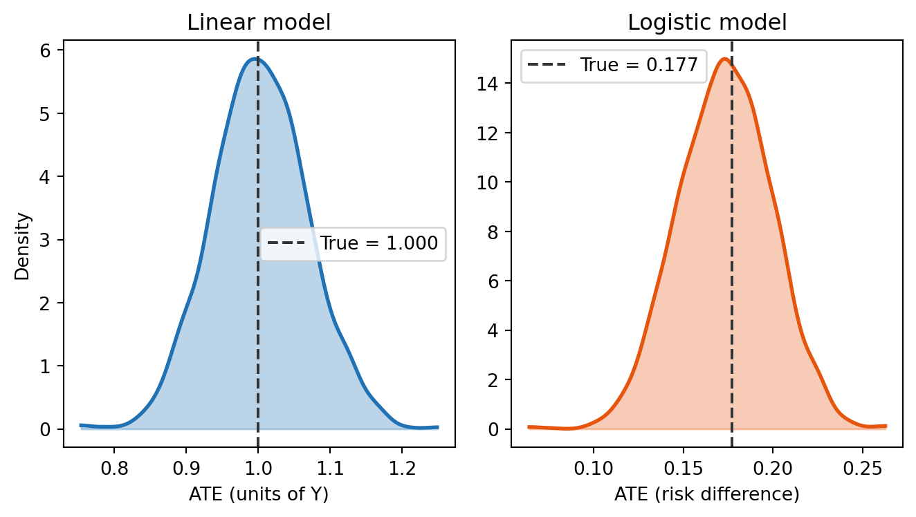

Figure 4: Posterior distributions of the estimated ATE for both models. Dashed lines show true values. The linear model’s ATE matches the coefficient (1.0); the logistic model’s ATE on the probability scale (~0.19) is far smaller than the log-odds coefficient (1.0).

Both ATEs are correctly recovered by do().

With confounding

In practice, treatment is rarely randomized. When a confounder Z affects both treatment assignment and the outcome, the naive comparison between treated and untreated groups is biased. With a nonlinear link function, the analyst faces two challenges simultaneously: adjusting for confounding and computing effects on the correct scale.

pathmc handles both in a single framework.

Figure 5: Confounded DAG: Z is a common cause of T and Y. The model must adjust for Z to identify the causal effect.

Z_conf = rng.normal(0, 1, size=n)
T_conf = rng.binomial(1, expit(0.8 * Z_conf)).astype(float)

logit_Y_conf = true_b0_log + true_bT_log * T_conf + true_bZ_log * Z_conf
Y_conf = rng.binomial(1, expit(logit_Y_conf)).astype(float)

df_conf = pd.DataFrame({"T": T_conf, "Z": Z_conf, "Y": Y_conf})

true_ate_conf = (
    expit(true_b0_log + true_bT_log + true_bZ_log * Z_conf)
    - expit(true_b0_log + true_bZ_log * Z_conf)
).mean()

naive_rd = Y_conf[T_conf == 1].mean() - Y_conf[T_conf == 0].mean()

print(f"Naive risk difference (biased): {naive_rd:.3f}")
print(f"True ATE (risk difference):     {true_ate_conf:.3f}")

Naive risk difference (biased): 0.391
True ATE (risk difference):     0.177

The naive comparison is biased upward because high-Z individuals are both more likely to be treated and more likely to have Y{=}1.

model_conf = pathmc.model(
    """
    T ~ Z
    Y ~ bT*T + bZ*Z
    """,
    data=df_conf,
    families={"T": "bernoulli", "Y": "bernoulli"},
)
model_conf.equations()

\begin{aligned} \beta_{T} &\sim \text{Normal}(mu=0,\, sigma=10) \\ \beta_{Y} &\sim \text{Normal}(mu=0,\, sigma=10) \\[6pt] \mu_{T} &= \beta_{0,\,T} + \mathrm{Z} \\ \mathrm{T} &\sim \text{Bernoulli}(\text{logit}^{-1}(\mu_{T})) \\ \mu_{Y} &= \beta_{0,\,Y} + bT \cdot \mathrm{T} + bZ \cdot \mathrm{Z} \\ \mathrm{Y} &\sim \text{Bernoulli}(\text{logit}^{-1}(\mu_{Y})) \end{aligned}

model_conf.fit(draws=500, tune=500, chains=4, random_seed=42)

ate_conf = model_conf.ate("Y", "T", values=(0.0, 1.0))
print(f"Naive (biased):  {naive_rd:.3f}    True ATE: {true_ate_conf:.3f}")
ate_conf

NUTS[nutpie]: [beta_Y, beta_T]

Naive (biased):  0.391    True ATE: 0.177

ATE of T on Y

Mean	0.21
94% HDI	[0.16, 0.26]
P(> 0)	1.00
Draws	2000

Methods: .hdi() .prob() .summary() .draws() .by_time() .dataset

By modelling the full DAG — including T ~ Z — pathmc adjusts for confounding through the structural equations and computes the ATE on the probability scale via g-computation.

ATT and ATU: subgroup-specific effects under nonlinearity

With a logistic link, the treatment effect varies across individuals because the same shift in log-odds produces different changes in probability depending on baseline risk. When treatment assignment is confounded — treated units have systematically different baseline risk than untreated units — the ATT and ATU diverge from the ATE.

true_att_conf = (
    expit(true_b0_log + true_bT_log + true_bZ_log * Z_conf[T_conf == 1])
    - expit(true_b0_log + true_bZ_log * Z_conf[T_conf == 1])
).mean()

true_atu_conf = (
    expit(true_b0_log + true_bT_log + true_bZ_log * Z_conf[T_conf == 0])
    - expit(true_b0_log + true_bZ_log * Z_conf[T_conf == 0])
).mean()

print(f"True ATE:  {true_ate_conf:.3f}  (average over all units)")
print(f"True ATT:  {true_att_conf:.3f}  (average over treated units)")
print(f"True ATU:  {true_atu_conf:.3f}  (average over untreated units)")
print(f"\nE[Z | T=1] = {Z_conf[T_conf == 1].mean():.2f}")
print(f"E[Z | T=0] = {Z_conf[T_conf == 0].mean():.2f}")

True ATE:  0.177  (average over all units)
True ATT:  0.177  (average over treated units)
True ATU:  0.177  (average over untreated units)

E[Z | T=1] = 0.36
E[Z | T=0] = -0.33

Treated units have higher Z on average (because Z drives treatment assignment), which means higher baseline probability of Y{=}1. On the logistic curve, these units are in a region with smaller marginal effects — so the ATT is slightly smaller than the ATU.

att_conf = model_conf.att("Y", "T", values=(0.0, 1.0))
atu_conf = model_conf.atu("Y", "T", values=(0.0, 1.0))

print(f"{'Estimand':<12} {'Estimate':>10} {'True':>10}")
print(f"{'ATE':<12} {ate_conf.mean():>10.3f} {true_ate_conf:>10.3f}")
print(f"{'ATT':<12} {att_conf.mean():>10.3f} {true_att_conf:>10.3f}")
print(f"{'ATU':<12} {atu_conf.mean():>10.3f} {true_atu_conf:>10.3f}")

Estimand       Estimate       True
ATE               0.211      0.177
ATT               0.207      0.177
ATU               0.213      0.177

Why ATT ≠ ATU in logistic models

Even without an explicit interaction term, the logistic link function creates implicit effect modification: the treatment effect on the probability scale depends on baseline risk, which varies with covariates. When treatment is confounded with those covariates, the treated and untreated groups occupy different regions of the response curve — and experience different average effects.

This is a second reason (beyond explicit interactions) why att() and atu() are important: nonlinear link functions make the treatment effect heterogeneous even when the structural equation has no interaction terms.

Mixed-family models: continuous and binary variables

So far, every model used a single family for the outcome. In practice, DAGs often mix continuous and binary variables — for example, a continuous mediator feeding into a binary outcome. pathmc handles this naturally through the families argument.

X_mix = rng.normal(size=n)
M_mix = 0.5 * X_mix + rng.normal(scale=0.5, size=n)

linear_mix = 0.3 + 0.8 * M_mix + 0.4 * X_mix
p_mix = 1 / (1 + np.exp(-linear_mix))
Y_mix = rng.binomial(1, p_mix, size=n).astype(float)

df_mix = pd.DataFrame({"X": X_mix, "M": M_mix, "Y": Y_mix})
print(f"P(Y=1) in data: {Y_mix.mean():.2f}")

P(Y=1) in data: 0.56

model_mix = pathmc.model(
    """
    M ~ a*X
    Y ~ b*M + c*X
    """,
    data=df_mix,
    families={"Y": "bernoulli"},
)
model_mix.equations()

\begin{aligned} \beta_{M} &\sim \text{Normal}(mu=0,\, sigma=10) \\ \sigma_{M} &\sim \text{HalfNormal}(sigma=1) \\ \beta_{Y} &\sim \text{Normal}(mu=0,\, sigma=10) \\[6pt] \mu_{M} &= \beta_{0,\,M} + a \cdot \mathrm{X} \\ \mathrm{M} &\sim \text{Normal}(\mu_{M},\, \sigma_{M}) \\ \mu_{Y} &= \beta_{0,\,Y} + b \cdot \mathrm{M} + c \cdot \mathrm{X} \\ \mathrm{Y} &\sim \text{Bernoulli}(\text{logit}^{-1}(\mu_{Y})) \end{aligned}

Variables not listed in families default to Gaussian. Here, M gets a Gaussian likelihood (with sigma), while Y gets a Bernoulli-logit likelihood (no sigma). The do() operator handles the link function automatically — it returns probabilities for Bernoulli variables and raw values for Gaussian ones.

model_mix.fit(draws=500, tune=500, chains=4, random_seed=42)

NUTS[nutpie]: [beta_Y, sigma_M, beta_M]

r0_mix = model_mix.do(set={"X": 0.0}, kind="mean")
r1_mix = model_mix.do(set={"X": 1.0}, kind="mean")

ate_mix = r1_mix - r0_mix
ate_mix

DoResult — 2000 draws, 3 variables

variable	mean	94% HDI
X	1.00	[1.00, 1.00]
M	0.48	[0.45, 0.51]
Y	0.19	[0.17, 0.22]

Methods: .draws() .mean() .hdi() .by_time() .dataset

With kind="predictive", residual noise is added at each step. For Gaussian variables this adds Normal noise; for Bernoulli variables the draws are binary (0 or 1) rather than probabilities. The predictive mean converges to the same value, but individual draws differ:

r_mean_mix = model_mix.do(set={"X": 1.0}, kind="mean")
r_pred_mix = model_mix.do(set={"X": 1.0}, kind="predictive")

print("kind='mean' vs kind='predictive' — E[Y | do(X=1)]:")
r_mean_mix

Sampling: [M, Y]

kind='mean' vs kind='predictive' — E[Y | do(X=1)]:

DoResult — 2000 draws, 3 variables

variable	mean	94% HDI
X	1.00	[1.00, 1.00]
M	0.49	[0.45, 0.54]
Y	0.77	[0.73, 0.81]

Methods: .draws() .mean() .hdi() .by_time() .dataset

r_pred_mix

DoResult — 2000 draws, 3 variables

variable	mean	94% HDI
X	1.00	[1.00, 1.00]
M	0.49	[-0.44, 1.43]
Y	0.77	[0.00, 1.00]

Methods: .draws() .mean() .hdi() .by_time() .dataset

Summary

In linear models, the ATE equals the coefficient on the treatment variable. The individual treatment effect is constant, and the covariate terms cancel in the counterfactual contrast.
In logistic models, the coefficient is on the log-odds scale and does not equal the ATE on the probability scale. The individual treatment effect varies with baseline covariates.
The odds ratio \exp(\beta_T) is a valid, constant summary of the treatment effect on the odds scale — but it is not a risk difference and is often harder to interpret for decisions.
The marginal effect at the mean (evaluating the ITE at \bar{Z}) overestimates the ATE due to Jensen’s inequality. The average marginal effect (AME) is the correct ATE.
G-computation — averaging counterfactual predictions over the covariate distribution — is the general method for computing the ATE from model parameters. It works for any link function.
pathmc’s do() operator implements g-computation automatically: it applies the correct link function, averages over the data, and propagates full posterior uncertainty.
When in doubt, use do(). It gives the right answer for linear, logistic, Poisson, or any other family — no manual transformation needed.

Reflection

In your own analyses:

When you fit a logistic regression for a binary outcome, do you report coefficients, odds ratios, or risk differences? Are your stakeholders interpreting them correctly?
If a clinical trial reports “the treatment doubled the odds of recovery” (OR = 2.0), how large is that effect on the probability of recovery? It depends on the baseline rate — the same nonlinearity issue this notebook demonstrates.
Could the treatment effects in your models vary across subgroups with different baseline risk? If so, the ATE might mask important heterogeneity worth examining with cate(), att(), or atu().