import numpy as np
import pandas as pd
import matplotlib.pyplot as plt
from scipy.special import expit
import pathmc

FIG_WIDTH = 7
FIG_HEIGHT = 4
COLOR_STRUCTURAL = "#2171b5"
COLOR_ADJUSTMENT = "#e6550d"
COLOR_TRUE = "#333333"
SEGMENT_COLORS = {0.0: "#2171b5", 1.0: "#e6550d", 2.0: "#31a354"}


def plot_hdi_line(x, samples, ax, color, hdi_prob=0.94, alpha=0.2, label=None):
    """Posterior mean with quantile band. samples shape (n_draws, n_points)."""
    lo_q = (1 - hdi_prob) / 2
    lower = np.quantile(samples, lo_q, axis=0)
    upper = np.quantile(samples, 1 - lo_q, axis=0)
    mean = samples.mean(axis=0)
    ax.fill_between(x, lower, upper, color=color, alpha=alpha, linewidth=0)
    ax.plot(x, mean, color=color, linewidth=2.5, label=label)
    return mean


TRUE_B0 = -0.3
TRUE_B_DOSE = 0.9
TRUE_B_INC = 0.5
TRUE_B_INT = 0.4
TRUE_B_SEG = 0.25

rng = np.random.default_rng(42)
n = 600Interventional Contrasts
Draw-wise contrasts (diff, ratio, lift) vs conditional covariates, unit-level distributions, and agreement with ate() on a Bernoulli outcome.
Goal: quantify how much conversion changes when ad spend moves from 0 to 1, and how that contrast varies with income and customer segment.
comparisons() applies diff, ratio, or lift draw-wise at each unit before averaging. On a Bernoulli GLM the contrast is a risk difference on the probability scale, not the log-odds coefficient. This notebook plots contrasts along a covariate grid, tabulates ratio and lift, checks agreement with ate(), and shows unit-level heterogeneity.
Prerequisites: Predictions, Comparisons, and Slopes; Treatment Effects with Non-Linear Models for coefficient vs ATE.
Setup
Contrast vs income, grouped by segment
comparisons() does not accept newdata, so we build contrasts on a datagrid() via two predictions() calls at the contrast levels. This is the same draw-wise logic comparisons() uses internally.
income_grid = np.linspace(-2.0, 2.0, 25)
contrast_rows = []

for seg in [0.0, 1.0, 2.0]:
    grid = pathmc.datagrid(df, income=income_grid, segment=[seg])
    grid = grid.assign(ad_spend=0.0)
    lo = scm.predictions("converted", set={"ad_spend": 0.0}, newdata=grid)
    hi = scm.predictions("converted", set={"ad_spend": 1.0}, newdata=grid)
    diff = hi.dataset["converted"] - lo.dataset["converted"]
    contrast_rows.append((seg, grid, diff))
Code
fig, axes = plt.subplots(1, 3, figsize=(FIG_WIDTH, FIG_HEIGHT * 1.2), sharey=True)
seg_labels = {0.0: "low", 1.0: "mid", 2.0: "high"}

for ax, (seg, grid, diff) in zip(axes, contrast_rows, strict=True):
    x = grid["income"].values
    samples = diff.stack(sample=("chain", "draw")).values.T
    color = SEGMENT_COLORS[seg]
    plot_hdi_line(x, samples, ax, color=color, alpha=0.2)
    true_y = true_contrast_diff(0.0, 1.0, x, seg)
    ax.plot(x, true_y, color=COLOR_TRUE, linestyle="--", linewidth=1.5)
    ax.set_title(f"segment={seg_labels[seg]}", fontweight="bold")
    ax.set_xlabel("income")
    ax.set_ylim(0, 0.6)

axes[0].set_ylabel("risk difference")
plt.tight_layout()
plt.show()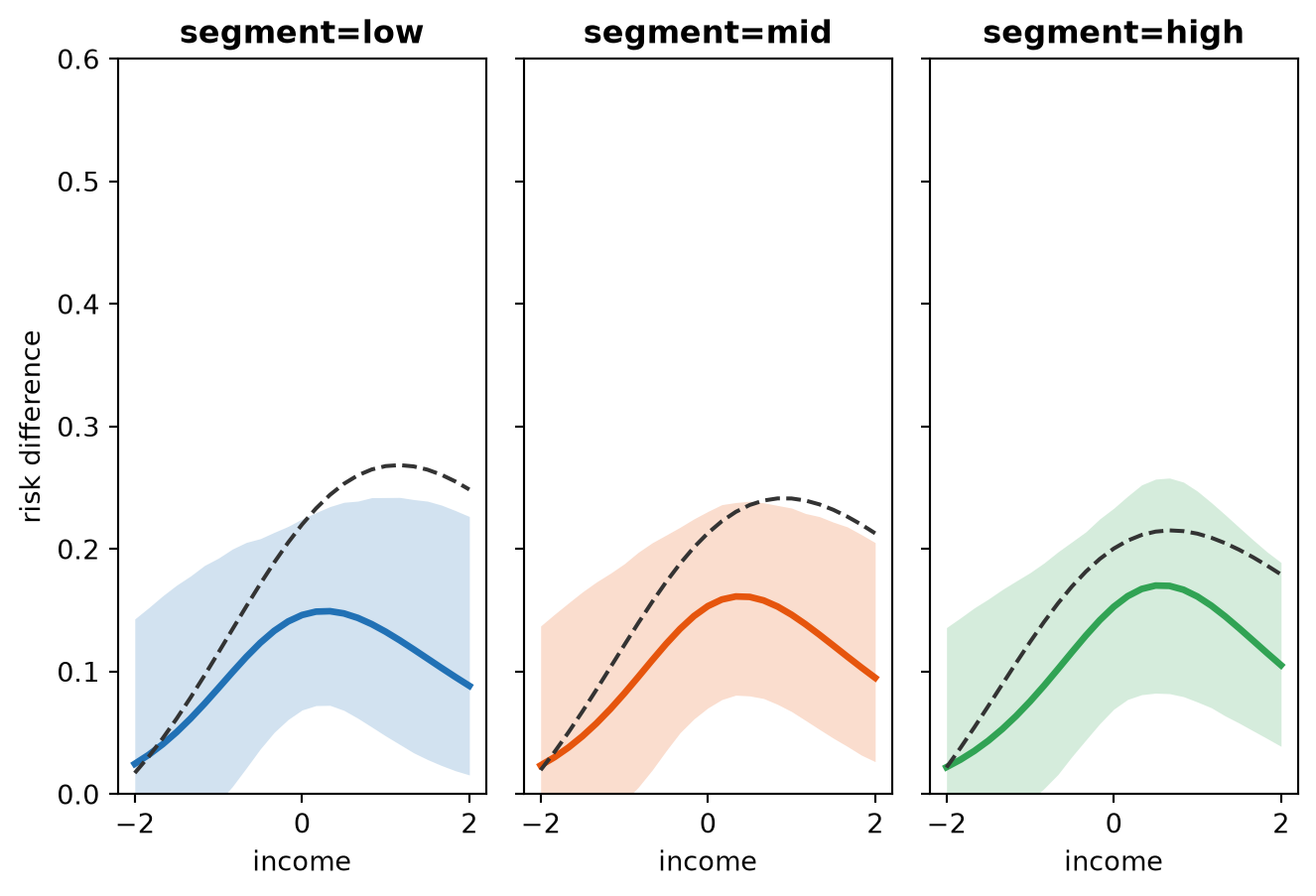
The contrast is not constant in income because of the ad_spend:income interaction on the logit scale.
Contrast table
table_rows = []
for seg in [0.0, 1.0, 2.0]:
    for inc in [-1.0, 0.0, 1.0]:
        comp = scm.comparisons(
            "converted",
            "ad_spend",
            contrast=(0.0, 1.0),
            comparison="diff",
            conditional={"income": inc, "segment": seg},
            average_by="all",
        )
        lo, hi = comp.hdi(prob=0.94)
        table_rows.append({
            "comparison": "diff",
            "contrast": "0 vs 1",
            "income": inc,
            "segment": int(seg),
            "mean": comp.mean(),
            "hdi_low": lo,
            "hdi_high": hi,
        })

pd.DataFrame(table_rows)| comparison | contrast | income | segment | mean | hdi_low | hdi_high | |
|---|---|---|---|---|---|---|---|
| 0 | diff | 0 vs 1 | -1.0 | 0 | 0.086565 | -0.013277 | 0.185380 |
| 1 | diff | 0 vs 1 | 0.0 | 0 | 0.146219 | 0.073074 | 0.228388 |
| 2 | diff | 0 vs 1 | 1.0 | 0 | 0.132569 | 0.038711 | 0.230003 |
| 3 | diff | 0 vs 1 | -1.0 | 1 | 0.082183 | -0.013506 | 0.177700 |
| 4 | diff | 0 vs 1 | 0.0 | 1 | 0.153489 | 0.073753 | 0.232575 |
| 5 | diff | 0 vs 1 | 1.0 | 1 | 0.146488 | 0.061364 | 0.226488 |
| 6 | diff | 0 vs 1 | -1.0 | 2 | 0.075714 | -0.007178 | 0.176648 |
| 7 | diff | 0 vs 1 | 0.0 | 2 | 0.152940 | 0.070985 | 0.234525 |
| 8 | diff | 0 vs 1 | 1.0 | 2 | 0.161327 | 0.074615 | 0.245942 |
Ratio and lift
ratio_lift_rows = []
for kind in ["diff", "ratio", "lift"]:
    result = scm.comparisons(
        "converted",
        "ad_spend",
        contrast=(0.0, 1.0),
        comparison=kind,
        average_by="all",
    )
    lo, hi = result.hdi(prob=0.94)
    ratio_lift_rows.append({
        "comparison": kind,
        "mean": result.mean(),
        "hdi_low": lo,
        "hdi_high": hi,
    })

pd.DataFrame(ratio_lift_rows)| comparison | mean | hdi_low | hdi_high | |
|---|---|---|---|---|
| 0 | diff | 0.127987 | 0.056774 | 0.200991 |
| 1 | ratio | 1.265986 | 1.096593 | 1.441829 |
| 2 | lift | 0.265986 | 0.096593 | 0.441829 |
Gold check: comparisons() matches ate()
With comparison="diff" and average_by="all", comparisons() and ate() share one implementation path.
comp = scm.comparisons(
    "converted",
    "ad_spend",
    contrast=(0.0, 1.0),
    comparison="diff",
    average_by="all",
)
ate = scm.ate("converted", "ad_spend", values=(0.0, 1.0))
print(f"comparisons mean: {comp.mean():.4f}")
print(f"ate mean:         {ate.mean():.4f}")
print(f"match: {np.isclose(comp.mean(), ate.mean())}")
comparisons mean: 0.1280
ate mean: 0.1280
match: TrueStructural vs adjustment ATE
Code
fig, ax = plt.subplots(figsize=(FIG_WIDTH, FIG_HEIGHT * 0.85))
for model, color, label in [
    (scm, COLOR_STRUCTURAL, "structural"),
    (adj, COLOR_ADJUSTMENT, "adjustment"),
]:
    if label == "structural":
        result = model.comparisons(
            "converted",
            "ad_spend",
            comparison="diff",
            average_by="all",
        )
    else:
        result = model.comparisons(comparison="diff", average_by="all")
    draws = result.draws()
    lo, hi = result.hdi(prob=0.94)
    ax.errorbar(
        label,
        result.mean(),
        yerr=[[result.mean() - lo], [hi - result.mean()]],
        fmt="o",
        color=color,
        markersize=10,
        capsize=5,
        linewidth=2,
    )

ax.set_ylabel("risk difference")
ax.axhline(
    true_contrast_diff(0, 1, income, segment).mean(),
    color=COLOR_TRUE,
    linestyle="--",
    label="true ATE",
)
ax.legend(frameon=False)
plt.tight_layout()
plt.show()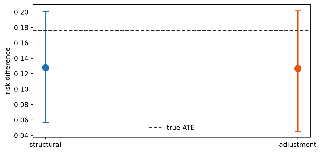
Unit-level contrasts
Set average_by=None to keep the unit dimension. The histogram supplements the grid plot; it does not replace it.
Code
unit_comp = scm.comparisons(
    "converted",
    "ad_spend",
    contrast=(0.0, 1.0),
    comparison="diff",
    average_by=None,
)
unit_draws = (
    unit_comp.dataset["converted"].stack(sample=("chain", "draw")).values.flatten()
)

fig, ax = plt.subplots(figsize=(FIG_WIDTH, FIG_HEIGHT * 0.85))
ax.hist(
    unit_draws, bins=40, density=True, alpha=0.7, color=COLOR_STRUCTURAL, edgecolor="k"
)
ax.axvline(
    unit_comp.mean(),
    color=COLOR_TRUE,
    linestyle="--",
    linewidth=2,
    label="posterior mean",
)
ax.set_xlabel("unit-level risk difference")
ax.set_ylabel("density")
ax.legend(frameon=False)
plt.tight_layout()
plt.show()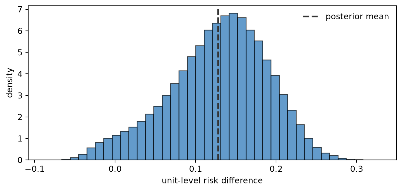
Summary
- Grid contrasts come from paired predictions() at contrast levels when you need a covariate axis.
diff,ratio, andliftare draw-wise transforms before averaging.comparisons(..., comparison="diff", average_by="all")matches ate() on the same contrast.- On a GLM the contrast varies with effect modifiers; a single ATE number hides that structure.
Next steps: Local Slopes; Conditional Predictions; Predictions, Comparisons, and Slopes; Estimation Approaches.
NoteReflection
Would your stakeholders report a single ATE or a curve of contrasts by customer segment? When would ratio or lift be more interpretable than a risk difference?