Many causal questions are about which group a unit belongs to rather than how much of something it received: which sales region a store sits in, which message variant a customer saw, which policy regime a country adopted. These predictors arrive as strings or pandas categoricals, and a regression cannot multiply a coefficient by "north". The usual workaround is to build indicator columns by hand:
dummies = pd.get_dummies(df["region"], drop_first=True) # region_south, region_west
That works until it doesn’t: the reference level is whichever value happens to sort first, new data with a missing or extra level silently produces a different set of columns, and an intervention such as “move every store to the south region” has to be translated by hand into flipping two indicator columns.
pathmc handles categorical predictors as a first-class part of the DSL instead. When you build a model, it detects string and categorical columns, expands each one into indicator columns using treatment coding, gives every non-reference level its own named coefficient, and — the part that matters for causal work — freezes the level set and reference so that predict() and do() can never silently recompute the coding on new data. Interventions then read the way you would say them: model.do(set={"region": "south"}).
This notebook walks through the full surface: automatic inference, explicit C() syntax, the two coding schemes, priors (including hierarchical shrinkage), interventions by label, prediction on new rows, and the boundaries of what is supported today.
This example assumes you are comfortable with the pathmc DSL (see Model Specification) and with the idea of an intervention as graph surgery (see The do() Operator). Everything else is introduced as we go.
Setup and simulated data
We simulate a store-level dataset with three sales regions and one continuous covariate. The data-generating process is deliberately simple so every estimate can be checked against a planted truth:
y_i = 1 + 0.5\,x_i + \delta_{\text{region}_i} + \varepsilon_i, \qquad \varepsilon_i \sim \mathcal{N}(0, 0.5^2)
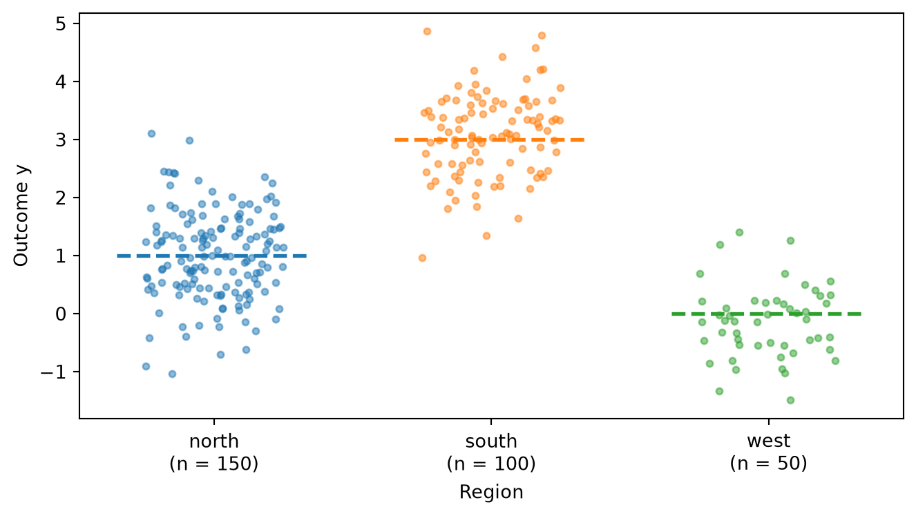
with region effects \delta_{\text{north}} = 0, \delta_{\text{south}} = 2, and \delta_{\text{west}} = -1. Group sizes are unequal on purpose — 150 north, 100 south, 50 west — because unbalanced groups are the norm in observational data and they matter later when we discuss priors.
import arviz as az
import matplotlib.pyplot as plt
import numpy as np
import pandas as pd
from scipy.stats import gaussian_kde

import pathmc
from pathmc import Prior

FIG_WIDTH = 7
FIG_HEIGHT = 4

COLORS = {"north": "#1f77b4", "south": "#ff7f0e", "west": "#2ca02c"}
LEVELS = ["north", "south", "west"]

TRUE_INTERCEPT = 1.0
TRUE_SLOPE_X = 0.5
TRUE_EFFECT = {"north": 0.0, "south": 2.0, "west": -1.0}
TRUE_GROUP_MEAN = {k: TRUE_INTERCEPT + v for k, v in TRUE_EFFECT.items()}

rng = np.random.default_rng(11)
region = np.repeat(LEVELS, [150, 100, 50])
rng.shuffle(region)
x = rng.normal(size=region.size)
y = (
    TRUE_INTERCEPT
    + TRUE_SLOPE_X * x
    + np.array([TRUE_EFFECT[r] for r in region])
    + rng.normal(scale=0.5, size=region.size)
)
df = pd.DataFrame({"y": y, "x": x, "region": region})
df.head()
|
y |
x |
region |
| 0 |
-0.614373 |
-0.941384 |
west |
| 1 |
1.339371 |
0.791763 |
north |
| 2 |
0.983779 |
-0.505302 |
north |
| 3 |
0.437651 |
-1.090653 |
north |
| 4 |
3.579574 |
0.365249 |
south |
The causal structure is the simplest possible: both region and x are exogenous causes of y, with no confounding between them (Figure 1).
Figure 2 shows the raw outcome by region. The group means sit close to the planted values of 1, 3, and 0, and the smaller west group is visibly noisier.
Code
fig, ax = plt.subplots(figsize=(FIG_WIDTH, FIG_HEIGHT))
for i, level in enumerate(LEVELS):
    mask = df["region"] == level
    jitter = rng.uniform(-0.25, 0.25, size=mask.sum())
    ax.scatter(i + jitter, df.loc[mask, "y"], s=12, alpha=0.5, color=COLORS[level])
    ax.hlines(
        TRUE_GROUP_MEAN[level],
        i - 0.35,
        i + 0.35,
        colors=COLORS[level],
        linestyles="--",
        linewidth=2,
    )
ax.set_xticks(range(len(LEVELS)))
ax.set_xticklabels([f"{lvl}\n(n = {(df['region'] == lvl).sum()})" for lvl in LEVELS])
ax.set_xlabel("Region")
ax.set_ylabel("Outcome y")
plt.tight_layout()
plt.show()
Treatment coding, in pictures
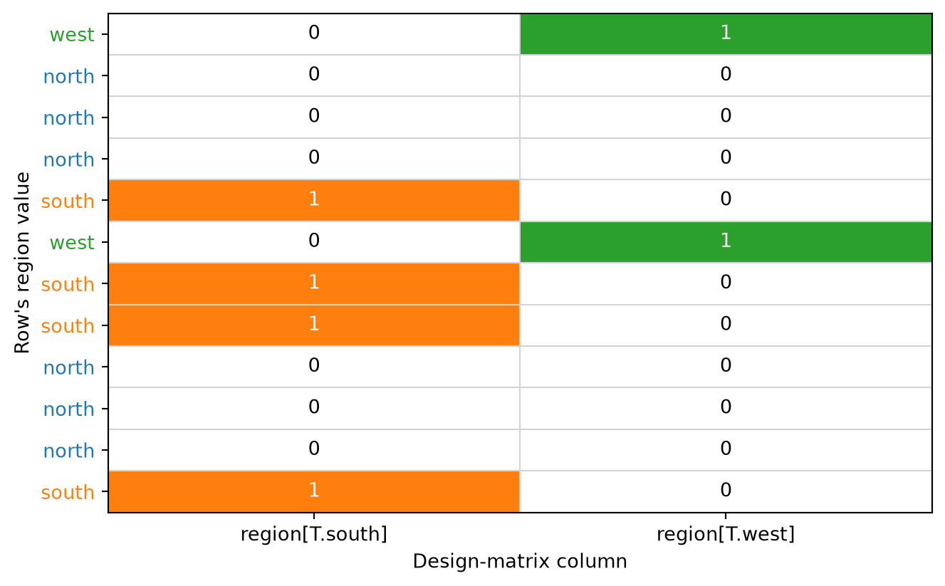
A regression cannot multiply a coefficient by the word “south”. The standard fix is treatment coding (also called dummy or reference coding). One level is chosen as the reference and absorbed into the intercept; every other level receives an indicator column that is 1 for rows in that level and 0 otherwise. For our three regions with north as reference, the linear predictor becomes
\mu_i = \beta_0 + \beta_x\,x_i + \beta_{\text{south}}\,\mathbb{1}[\text{region}_i = \text{south}] + \beta_{\text{west}}\,\mathbb{1}[\text{region}_i = \text{west}]
so that \beta_0 is the expected outcome for a north store at x = 0, and \beta_{\text{south}} and \beta_{\text{west}} are the differences from north. Each row of the data therefore maps to one of three indicator patterns:
| north (reference) |
0 |
0 |
\beta_0 |
| south |
1 |
0 |
\beta_0 + \beta_{\text{south}} |
| west |
0 |
1 |
\beta_0 + \beta_{\text{west}} |
Figure 3 shows this for the first rows of our data. The T. in the column names is the conventional marker for a treatment contrast against the reference.
Code
preview = pathmc.model("y ~ x + region", data=df).design("y")
indicator_cols = [c for c in preview.columns if c.startswith("region[")]
block = preview[indicator_cols].head(12).to_numpy()
labels = df["region"].head(12).tolist()

from matplotlib.colors import to_rgb

column_levels = [c[len("region[T.") : -1] for c in indicator_cols]
rgb = np.ones(block.shape + (3,))
for c, level in enumerate(column_levels):
    rgb[block[:, c] == 1, c, :] = to_rgb(COLORS[level])

fig, ax = plt.subplots(figsize=(FIG_WIDTH, FIG_HEIGHT * 1.1))
ax.imshow(rgb, aspect="auto")
for r in range(block.shape[0]):
    for c in range(block.shape[1]):
        ax.text(
            c,
            r,
            int(block[r, c]),
            ha="center",
            va="center",
            color="white" if block[r, c] else "black",
            fontsize=10,
        )
ax.set_xticks(np.arange(-0.5, len(indicator_cols)), minor=True)
ax.set_yticks(np.arange(-0.5, len(labels)), minor=True)
ax.grid(which="minor", color="lightgray", linewidth=0.8)
ax.tick_params(which="minor", length=0)
ax.set_xticks(range(len(indicator_cols)))
ax.set_xticklabels(indicator_cols)
ax.set_yticks(range(len(labels)))
ax.set_yticklabels(labels)
for tick, label in zip(ax.get_yticklabels(), labels):
    tick.set_color(COLORS[label])
ax.set_xlabel("Design-matrix column")
ax.set_ylabel("Row's region value")
plt.tight_layout()
plt.show()
Automatic inference from the data
The simplest specification lists the column like any other predictor. pathmc inspects the data at build time and treats the column as categorical because it holds strings.
model = pathmc.model("y ~ x + region", data=df)
model.equations()
\begin{aligned}
\beta_{y} &\sim \text{Normal}(mu=0,\, sigma=10) \\
\sigma_{y} &\sim \text{HalfNormal}(sigma=1) \\
\beta_{y,region} &\sim \text{Normal}(mu=0,\, sigma=10)
\\[6pt]
\mu_{y} &= \beta_{0,\,y} + \mathrm{x} + \operatorname{C}(\mathrm{region};\,\mathrm{ref}=north;\,\mathrm{levels}=\{north, south, west\}) \\
\mathrm{y} &\sim \text{Normal}(\mu_{y},\, \sigma_{y})
\end{aligned}
The equation display is a term-level shorthand: x stands for the slope term \beta_x x_i, and C(region; ...) stands for the whole block of level indicators and their coefficients. What it records is everything the compiler froze about the categorical: the variable, the reference level, and the full ordered level set. The design matrix confirms the indicator columns sit alongside the continuous predictor:
|
Intercept |
x |
region[T.south] |
region[T.west] |
| 0 |
1.0 |
-0.941384 |
0.0 |
1.0 |
| 1 |
1.0 |
0.791763 |
0.0 |
0.0 |
| 2 |
1.0 |
-0.505302 |
0.0 |
0.0 |
| 3 |
1.0 |
-1.090653 |
0.0 |
0.0 |
| 4 |
1.0 |
0.365249 |
1.0 |
0.0 |
pathmc infers a plain term as categorical when the column is any of:
- a pandas
Categorical dtype (declared category order is respected — see below),
- a pandas
StringDtype column,
- an
object column whose non-missing values are strings or bytes.
An object column that merely holds numbers (for example, integers stored as Python objects) stays continuous. Integer and float columns are always continuous unless you wrap them in C(). Polars and other narwhals-compatible frames are converted to pandas for this inspection, so the same rules apply.
Parameter names and coordinates
Categorical coefficients live in their own vector, separate from the equation’s flat beta_y vector that holds the intercept and continuous slopes. The name is always beta_{outcome}_{variable}, and the vector carries an xarray coordinate {outcome}_{variable}_levels whose labels are the represented levels:
\begin{aligned}
\beta_{y} &\sim \text{Normal}(mu=0,\, sigma=10) \\
\sigma_{y} &\sim \text{HalfNormal}(sigma=1) \\
\beta_{y,region} &\sim \text{Normal}(mu=0,\, sigma=10)
\end{aligned}
{name: list(values) for name, values in model.pymc_model.coords.items()}
{'y_predictors': ['Intercept', 'x'], 'y_region_levels': ['south', 'west']}
Because beta_y_region is indexed by level name rather than position, posteriors read naturally in summary() and ArviZ without ever reconstructing patsy’s column order.
Fit and check against the truth
idata = model.fit(random_seed=42)
az.summary(
    idata,
    var_names=["beta_y", "beta_y_region", "sigma_y"],
    ci_prob=0.94,
    ci_kind="hdi",
    round_to=2,
)
NUTS[nutpie]: [beta_y_region, beta_y, sigma_y]
|
mean |
sd |
hdi94_lb |
hdi94_ub |
ess_bulk |
ess_tail |
r_hat |
mcse_mean |
mcse_sd |
| beta_y[Intercept] |
1.01 |
0.04 |
0.93 |
1.09 |
2149.09 |
2506.59 |
1.0 |
0.0 |
0.0 |
| beta_y[x] |
0.51 |
0.03 |
0.45 |
0.57 |
4359.37 |
3189.37 |
1.0 |
0.0 |
0.0 |
| beta_y_region[south] |
1.96 |
0.07 |
1.83 |
2.09 |
2242.07 |
2683.62 |
1.0 |
0.0 |
0.0 |
| beta_y_region[west] |
-1.07 |
0.09 |
-1.23 |
-0.90 |
2728.12 |
2704.13 |
1.0 |
0.0 |
0.0 |
| sigma_y |
0.53 |
0.02 |
0.49 |
0.57 |
4305.59 |
3168.37 |
1.0 |
0.0 |
0.0 |
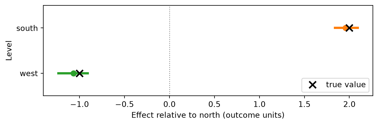
Before going further we verify that the workflow recovers the planted values. Figure 4 puts the posterior for each region contrast next to its truth: \beta_{\text{south}} = 2 and \beta_{\text{west}} = -1.
Code
def forest_by_level(ax, post, coord, truth, colors, offset=0.0, label=None):
    """Horizontal forest plot of one coefficient vector keyed by level."""
    levels = list(post[coord].values)
    for i, level in enumerate(levels):
        draws = post.sel({coord: level}).values.ravel()
        lo, hi = az.hdi(draws, prob=0.94)
        ax.plot([lo, hi], [i + offset, i + offset], color=colors[level], lw=3)
        ax.plot(
            draws.mean(),
            i + offset,
            "o",
            color=colors[level],
            ms=7,
            label=label if i == 0 else None,
        )
        if truth is not None:
            ax.plot(
                truth[level],
                i + offset,
                "x",
                color="black",
                ms=9,
                mew=2,
                label="true value" if i == 0 and label is None else None,
            )
    ax.set_yticks(range(len(levels)))
    ax.set_yticklabels(levels)
    ax.set_ylim(len(levels) - 0.5, -0.5)


fig, ax = plt.subplots(figsize=(FIG_WIDTH, FIG_HEIGHT * 0.6))
forest_by_level(
    ax, idata.posterior["beta_y_region"], "y_region_levels", TRUE_EFFECT, COLORS
)
ax.axvline(0, color="gray", lw=1, ls=":")
ax.set_xlabel("Effect relative to north (outcome units)")
ax.set_ylabel("Level")
ax.legend(loc="lower right")
plt.tight_layout()
plt.show()
Takeaway: the posteriors bracket the planted contrasts, and uncertainty scales with group size exactly as it should. The rest of the notebook builds on this validated fit.
Choosing the reference level with C()
Automatic inference picks the first level in sorted order (north) as the reference. That is often not the comparison you care about. The explicit C() syntax makes every coding decision visible in the specification:
C(variable, reference=<level>, prior='independent' | 'hierarchical')
Here we ask for south as the baseline. The design columns change accordingly:
model_south = pathmc.model("y ~ x + C(region, reference='south')", data=df)
model_south.design("y").head(3)
|
Intercept |
x |
region[T.north] |
region[T.west] |
| 0 |
1.0 |
-0.941384 |
0.0 |
1.0 |
| 1 |
1.0 |
0.791763 |
1.0 |
0.0 |
| 2 |
1.0 |
-0.505302 |
1.0 |
0.0 |
idata_south = model_south.fit(random_seed=42)
az.summary(
    idata_south,
    var_names=["beta_y_region"],
    ci_prob=0.94,
    ci_kind="hdi",
    round_to=2,
)
NUTS[nutpie]: [beta_y_region, beta_y, sigma_y]
|
mean |
sd |
hdi94_lb |
hdi94_ub |
ess_bulk |
ess_tail |
r_hat |
mcse_mean |
mcse_sd |
| beta_y_region[north] |
-1.96 |
0.07 |
-2.09 |
-1.83 |
1816.04 |
1768.23 |
1.0 |
0.0 |
0.0 |
| beta_y_region[west] |
-3.03 |
0.09 |
-3.20 |
-2.85 |
2338.47 |
2556.87 |
1.0 |
0.0 |
0.0 |
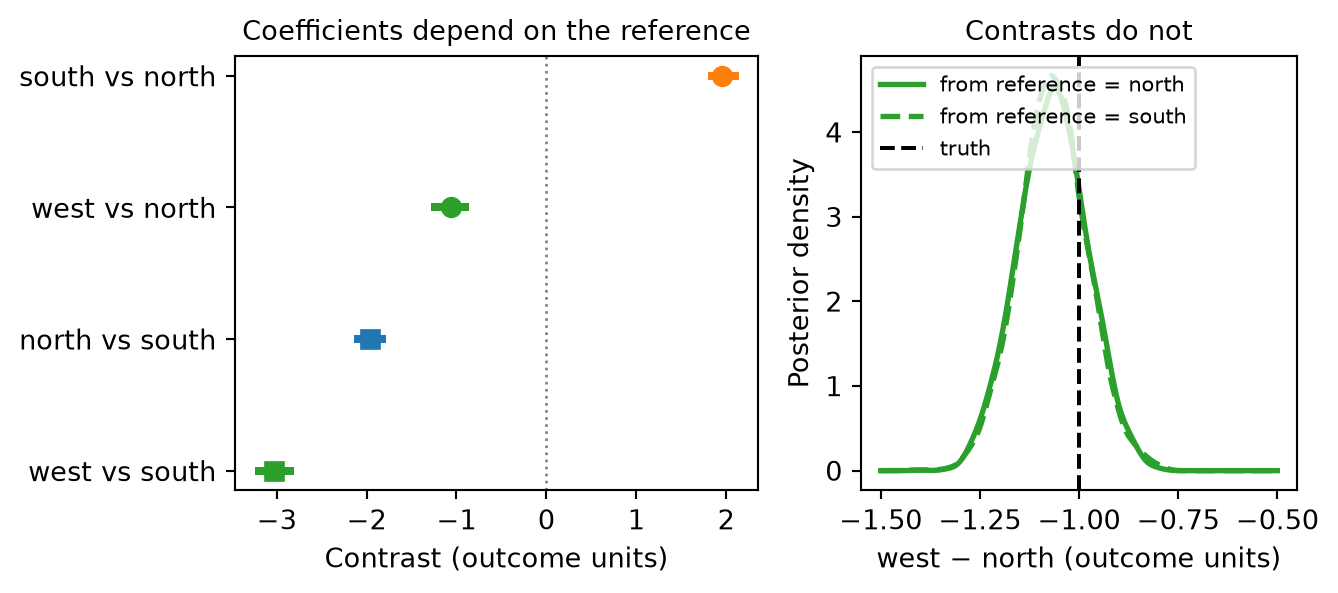
The coefficients now read “north relative to south” (-2) and “west relative to south” (-3). It is important to see that this is a reparametrization, not a different model: the fitted values, the residual scale, and any pairwise contrast are the same whichever reference you pick. Figure 5 demonstrates this by computing the west-minus-north contrast from both fits. Under reference='north' it is simply \beta_{\text{west}}; under reference='south' it is \beta_{\text{west}} - \beta_{\text{north}}.
Code
post_n = idata.posterior["beta_y_region"]
post_s = idata_south.posterior["beta_y_region"]
west_minus_north_ref_n = post_n.sel(y_region_levels="west").values.ravel()
west_minus_north_ref_s = (
    post_s.sel(y_region_levels="west") - post_s.sel(y_region_levels="north")
).values.ravel()

fig, (ax_l, ax_r) = plt.subplots(
    1, 2, figsize=(FIG_WIDTH, FIG_HEIGHT * 0.8), gridspec_kw={"width_ratios": [1.2, 1]}
)
rows = [
    ("south vs north", post_n.sel(y_region_levels="south"), "south", "o"),
    ("west vs north", post_n.sel(y_region_levels="west"), "west", "o"),
    ("north vs south", post_s.sel(y_region_levels="north"), "north", "s"),
    ("west vs south", post_s.sel(y_region_levels="west"), "west", "s"),
]
for i, (name, da, level, marker) in enumerate(rows):
    draws = da.values.ravel()
    lo, hi = az.hdi(draws, prob=0.94)
    ax_l.plot([lo, hi], [i, i], color=COLORS[level], lw=3)
    ax_l.plot(draws.mean(), i, marker, color=COLORS[level], ms=7)
ax_l.set_yticks(range(len(rows)))
ax_l.set_yticklabels([r[0] for r in rows])
ax_l.invert_yaxis()
ax_l.axvline(0, color="gray", lw=1, ls=":")
ax_l.set_xlabel("Contrast (outcome units)")
ax_l.set_title("Coefficients depend on the reference", fontsize=10)

grid = np.linspace(-1.5, -0.5, 300)
for draws, ls, label in [
    (west_minus_north_ref_n, "-", "from reference = north"),
    (west_minus_north_ref_s, "--", "from reference = south"),
]:
    ax_r.plot(
        grid, gaussian_kde(draws)(grid), color=COLORS["west"], ls=ls, lw=2, label=label
    )
ax_r.axvline(TRUE_EFFECT["west"], color="black", ls="--", lw=1.5, label="truth")
ax_r.set_xlabel("west − north (outcome units)")
ax_r.set_ylabel("Posterior density")
ax_r.set_title("Contrasts do not", fontsize=10)
ax_r.legend(fontsize=8, loc="upper left")
plt.tight_layout()
plt.show()
Pick the level you want the other coefficients to be compared against — usually a control condition, a status-quo policy, or the largest group (which gives the intercept the tightest posterior). If no single baseline is natural, use the intercept-free coding described next and compute contrasts afterwards.
Cell-means coding with 0 +
Dropping the intercept with 0 + changes the coding scheme. With no intercept to absorb a baseline, every level gets its own indicator column and coefficient, and the column names lose the T. marker:
model_cells = pathmc.model("y ~ 0 + x + region", data=df)
model_cells.design("y").head(3)
|
x |
region[north] |
region[south] |
region[west] |
| 0 |
-0.941384 |
0.0 |
0.0 |
1.0 |
| 1 |
0.791763 |
1.0 |
0.0 |
0.0 |
| 2 |
-0.505302 |
1.0 |
0.0 |
0.0 |
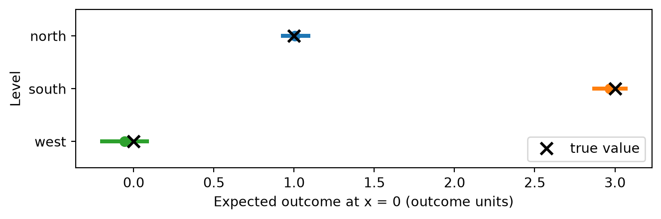
Each coefficient is now the expected outcome for that level at x = 0 — a cell mean — rather than a difference from a reference. Since the true group means are 1, 3, and 0, that is what the fit should return (Figure 6).
idata_cells = model_cells.fit(random_seed=42)
az.summary(
    idata_cells,
    var_names=["beta_y_region"],
    ci_prob=0.94,
    ci_kind="hdi",
    round_to=2,
)
NUTS[nutpie]: [beta_y_region, beta_y, sigma_y]
|
mean |
sd |
hdi94_lb |
hdi94_ub |
ess_bulk |
ess_tail |
r_hat |
mcse_mean |
mcse_sd |
| beta_y_region[north] |
1.01 |
0.04 |
0.93 |
1.09 |
7862.28 |
2907.53 |
1.0 |
0.0 |
0.0 |
| beta_y_region[south] |
2.97 |
0.05 |
2.87 |
3.06 |
6128.45 |
3659.72 |
1.0 |
0.0 |
0.0 |
| beta_y_region[west] |
-0.06 |
0.08 |
-0.20 |
0.08 |
6675.37 |
3207.78 |
1.0 |
0.0 |
0.0 |
Code
fig, ax = plt.subplots(figsize=(FIG_WIDTH, FIG_HEIGHT * 0.6))
forest_by_level(
    ax,
    idata_cells.posterior["beta_y_region"],
    "y_region_levels",
    TRUE_GROUP_MEAN,
    COLORS,
)
ax.set_xlabel("Expected outcome at x = 0 (outcome units)")
ax.set_ylabel("Level")
ax.legend(loc="lower right")
plt.tight_layout()
plt.show()
The two coding schemes are summarized below. Both are full rank; the choice is about which quantities you want the coefficients to represent directly.
y ~ region (intercept present) |
one per non-reference level |
region[T.south], region[T.west] |
difference from the reference level |
y ~ 0 + region (intercept suppressed) |
one per level |
region[north], region[south], region[west] |
expected outcome for that level |
Exactly one term per equation supplies the baseline. With 0 + that is the first categorical; a second categorical in the same equation (y ~ 0 + region + channel) is treatment coded against it, so the design never becomes collinear.
Priors on level effects
Independent priors (default)
By default every categorical coefficient gets an independent Normal(0, 10) prior — the same weakly informative default as ordinary slopes. You override it by name, exactly like other coefficients. A scalar prior is broadcast across levels:
model_prior = pathmc.model("y ~ x + region", data=df)
model_prior.set_priors({"beta_y_region": Prior("Normal", mu=0, sigma=2)})
model_prior.priors()
\begin{aligned}
\beta_{y} &\sim \text{Normal}(mu=0,\, sigma=10) \\
\sigma_{y} &\sim \text{HalfNormal}(sigma=1) \\
\beta_{y,region} &\sim \text{Normal}(mu=0,\, sigma=2)
\end{aligned}
To give different levels different priors, pass vectors and name the level dimension. The order follows the coordinate shown by model.pymc_model.coords, which is the non-reference levels in their frozen order — here south then west. The values below are purely illustrative (a mildly informative belief that south is above the reference and west is below it), not the simulated truths:
model_prior.set_priors({
    "beta_y_region": Prior(
        "Normal", mu=[1.0, -0.5], sigma=[1.0, 1.0], dims=("y_region_levels",)
    )
})
model_prior.priors()
\begin{aligned}
\beta_{y} &\sim \text{Normal}(mu=0,\, sigma=10) \\
\sigma_{y} &\sim \text{HalfNormal}(sigma=1) \\
\beta_{y,region} &\sim \text{Normal}(mu=[ 1. -0.5],\, sigma=[1. 1.])
\end{aligned}
When levels come from C() on an integer column, coordinate order is the string sort of the codes: twelve stores coded 1..12 are ordered 1, 10, 11, 12, 2, 3, .... Always read the order from model.pymc_model.coords before writing a per-level vector prior, or declare the column as a pandas Categorical with the order you want.
Hierarchical shrinkage
With a handful of well-populated levels, independent priors are fine. Categorical predictors often have many levels with very unequal counts — dozens of stores, hundreds of postcodes — and then the sparse levels produce noisy, overconfident-looking estimates. A prior='hierarchical' term places a shared population distribution over the level effects:
\beta_{\ell} \sim \mathcal{N}(\mu_\beta, \sigma_\beta), \qquad \mu_\beta \sim \mathcal{N}(0, 10), \qquad \sigma_\beta \sim \text{HalfNormal}(1)
so that levels with little data are pulled towards the population mean by an amount the data itself decides through \sigma_\beta. Every level is pooled — there is no reference level to escape shrinkage — so the term carries its own population mean and takes over the intercept’s role: the linear predictor below has no separate Intercept, and mu_beta_{outcome}_{variable} and sigma_beta_{outcome}_{variable} are the two named hyperparameters:
hier_model = pathmc.model("y ~ x + C(region, prior='hierarchical')", data=df)
hier_model.equations()
\begin{aligned}
\beta_{y} &\sim \text{Normal}(mu=0,\, sigma=10) \\
\sigma_{y} &\sim \text{HalfNormal}(sigma=1) \\
\sigma_{beta,y,region} &\sim \text{HalfNormal}(sigma=1) \\
\mu_{beta,y,region} &\sim \text{Normal}(mu=0,\, sigma=10) \\
\beta_{y,region} &\sim \text{Normal}(mu\_beta\_y\_region,\, sigma\_beta\_y\_region)
\\[6pt]
\mu_{y} &= \mathrm{x} + \operatorname{C}(\mathrm{region};\,\mathrm{prior}=\mathrm{hierarchical};\,\mathrm{levels}=\{north, south, west\}) \\
\mathrm{y} &\sim \text{Normal}(\mu_{y},\, \sigma_{y})
\end{aligned}
\begin{aligned}
\beta_{y} &\sim \text{Normal}(mu=0,\, sigma=10) \\
\sigma_{y} &\sim \text{HalfNormal}(sigma=1) \\
\sigma_{beta,y,region} &\sim \text{HalfNormal}(sigma=1) \\
\mu_{beta,y,region} &\sim \text{Normal}(mu=0,\, sigma=10) \\
\beta_{y,region} &\sim \text{Normal}(mu\_beta\_y\_region,\, sigma\_beta\_y\_region)
\end{aligned}
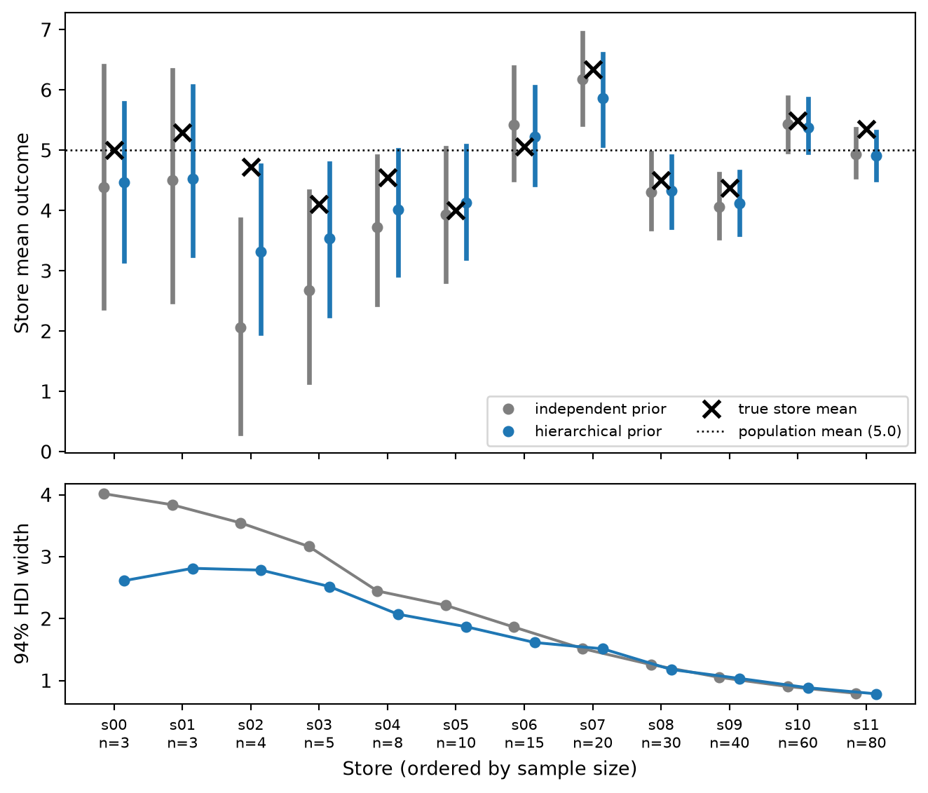
To see the effect, we simulate a second dataset with twelve stores whose sample sizes range from 3 to 80, and compare the independent and hierarchical fits using cell-means coding so every store gets a directly comparable coefficient.
store_rng = np.random.default_rng(7)
N_PER_STORE = [3, 3, 4, 5, 8, 10, 15, 20, 30, 40, 60, 80]
STORE_IDS = [f"s{i:02d}" for i in range(len(N_PER_STORE))]
TRUE_STORE_MEAN = dict(zip(STORE_IDS, 5.0 + store_rng.normal(scale=1.0, size=12)))

store = np.repeat(STORE_IDS, N_PER_STORE)
stores_df = pd.DataFrame({
    "store": store,
    "y": np.array([TRUE_STORE_MEAN[s] for s in store])
    + store_rng.normal(scale=2.0, size=store.size),
})

independent = pathmc.model("y ~ 0 + C(store)", data=stores_df)
hierarchical = pathmc.model("y ~ 0 + C(store, prior='hierarchical')", data=stores_df)
idata_ind = independent.fit(random_seed=7)
idata_hier = hierarchical.fit(random_seed=7)
NUTS[nutpie]: [beta_y_store, sigma_y]
NUTS[nutpie]: [sigma_beta_y_store, mu_beta_y_store, beta_y_store, sigma_y]
Code
COLOR_IND = "#7f7f7f"
COLOR_HIER = "#1f77b4"

fig, (ax_top, ax_bot) = plt.subplots(
    2,
    1,
    figsize=(FIG_WIDTH, FIG_HEIGHT * 1.5),
    sharex=True,
    gridspec_kw={"height_ratios": [2, 1]},
)
positions = np.arange(len(STORE_IDS))
for post, color, offset, label in [
    (idata_ind.posterior["beta_y_store"], COLOR_IND, -0.15, "independent prior"),
    (idata_hier.posterior["beta_y_store"], COLOR_HIER, 0.15, "hierarchical prior"),
]:
    widths = []
    for i, s in enumerate(STORE_IDS):
        draws = post.sel(y_store_levels=s).values.ravel()
        lo, hi = az.hdi(draws, prob=0.94)
        widths.append(hi - lo)
        ax_top.plot([i + offset, i + offset], [lo, hi], color=color, lw=2.5)
        ax_top.plot(
            i + offset,
            draws.mean(),
            "o",
            color=color,
            ms=5,
            label=label if i == 0 else None,
        )
    ax_bot.plot(positions + offset, widths, "o-", color=color, ms=5, label=label)

ax_top.plot(
    positions,
    [TRUE_STORE_MEAN[s] for s in STORE_IDS],
    "x",
    color="black",
    ms=9,
    mew=2,
    label="true store mean",
    zorder=5,
)
ax_top.axhline(5.0, color="black", ls=":", lw=1, label="population mean (5.0)")
ax_top.set_ylabel("Store mean outcome")
ax_top.legend(fontsize=8, ncol=2, loc="lower right")

ax_bot.set_ylabel("94% HDI width")
ax_bot.set_xlabel("Store (ordered by sample size)")
ax_bot.set_xticks(positions)
ax_bot.set_xticklabels(
    [f"{s}\nn={n}" for s, n in zip(STORE_IDS, N_PER_STORE)], fontsize=8
)
plt.tight_layout()
plt.show()
Takeaway: for the three stores with only three or four observations, the independent posterior is wide and jumps towards whatever noise those few rows contained, while the hierarchical posterior is pulled towards the population mean and is markedly narrower. From roughly 15 observations upward the two agree, because the data then dominate the prior. This is partial pooling working as intended, and it is why prior='hierarchical' is the recommended choice whenever a categorical has many or sparsely observed levels.
Partial pooling trades a little bias for a lot of variance reduction. A genuinely unusual level with very few observations will be pulled towards the crowd. If you have strong prior knowledge that one level is different, encode it through the hyperprior on sigma_beta_* (a larger scale permits more spread) or give that level its own independent term.
Intervening by label
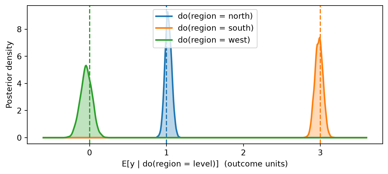
Treatment coding is an internal representation. When you intervene you speak in labels, and pathmc rebuilds the indicator matrix for you: setting the reference selects the all-zero row, setting any other level activates its indicator. The do() operator applies this to every row and averages over the remaining covariates, which is g-computation of the interventional mean E[y \mid do(\text{region} = \ell)].
interventions = {level: model.do(set={"region": level}) for level in LEVELS}
{level: round(r.mean("y"), 2) for level, r in interventions.items()}
{'north': 1.02, 'south': 2.98, 'west': -0.04}
Code
fig, ax = plt.subplots(figsize=(FIG_WIDTH, FIG_HEIGHT * 0.8))
grid = np.linspace(-0.6, 3.6, 500)
for level in LEVELS:
    draws = interventions[level].draws("y")
    density = gaussian_kde(draws)(grid)
    ax.fill_between(grid, density, alpha=0.3, color=COLORS[level])
    ax.plot(grid, density, color=COLORS[level], lw=2, label=f"do(region = {level})")
    ax.axvline(TRUE_GROUP_MEAN[level], color=COLORS[level], ls="--", lw=1.5)
ax.set_xlabel("E[y | do(region = level)]  (outcome units)")
ax.set_ylabel("Posterior density")
ax.legend(loc="upper center")
plt.tight_layout()
plt.show()
Contrasts between levels
Subtracting two DoResult objects gives the posterior of the causal contrast, draw by draw. The ate() wrapper does the same in one call and returns an EstimandResult that knows its outcome:
contrast = interventions["south"] - interventions["north"]
print(
    f"E[y | do(south)] − E[y | do(north)] = {contrast.mean('y'):.2f}, "
    f"94% HDI {np.round(contrast.hdi('y'), 2)}"
)
model.ate("y", "region", values=("north", "south"))
E[y | do(south)] − E[y | do(north)] = 1.96, 94% HDI [1.84 2.09]
ATE of region on y
| Mean | 1.96 |
| 94% HDI | [1.84, 2.09] |
| P(> 0) | 1.00 |
| Draws | 4000 |
The true value is \delta_{\text{south}} - \delta_{\text{north}} = 2. Any pair of labels works, including pairs that do not involve the reference:
model.ate("y", "region", values=("west", "south"))
ATE of region on y
| Mean | 3.02 |
| 94% HDI | [2.86, 3.20] |
| P(> 0) | 1.00 |
| Draws | 4000 |
Mixing categorical and continuous interventions
A single do() call can set a categorical label alongside a numeric value. Four query methods accept labels today — do(), ate(), prob(), and cate() — as interventions (set=, values=) and as conditions (condition=); the remaining helpers are listed under the boundaries at the end of this page:
both = model.do(set={"region": "west", "x": 1.0})
print(
    f"E[y | do(region = west, x = 1)] = {both.mean('y'):.2f}  "
    f"(truth {TRUE_INTERCEPT + TRUE_SLOPE_X * 1.0 + TRUE_EFFECT['west']:.2f})"
)

print(
    f"P(y > 2 | do(region = south)) = {model.prob('y > 2', set={'region': 'south'}):.2f}"
)

model.cate("y", "x", values=(0.0, 1.0), condition={"region": "south"})
E[y | do(region = west, x = 1)] = 0.45  (truth 0.50)
P(y > 2 | do(region = south)) = 0.91
CATE of x on y
| Mean | 0.51 |
| 94% HDI | [0.45, 0.57] |
| P(> 0) | 1.00 |
| Draws | 4000 |
kind="predictive" propagates the residual noise as well, giving the posterior predictive distribution of an individual store’s outcome under the intervention rather than the interventional mean:
predictive = model.do(set={"region": "south"}, kind="predictive")
print(
    f"mean {predictive.mean('y'):.2f}, 94% interval {np.round(predictive.hdi('y'), 2)}"
)
mean 2.98, 94% interval [1.58 4.36]
The predictive interval is far wider than the interval on the mean in Figure 8 because it includes the \sigma_y = 0.5 observation noise.
Predicting for new rows
predict(data=...) runs posterior predictive sampling with replacement predictor values. Categorical columns in the new frame are encoded with the fitted level set and reference, so it does not matter whether the levels arrive in a different row order or whether a level happens to be absent from the new frame. Here we move every store one region along a fixed cycle, so every row’s region changes:
NEXT_REGION = {"north": "south", "south": "west", "west": "north"}
new_rows = df.assign(region=df["region"].map(NEXT_REGION))
pp = model.predict(data=new_rows, extend_inferencedata=False, progressbar=False)

predicted_mean = pp.posterior_predictive["y"].mean(("chain", "draw")).values
pd.DataFrame({
    "region": new_rows["region"],
    "x": new_rows["x"].round(2),
    "predicted mean": predicted_mean.round(2),
    "true mean": (
        TRUE_INTERCEPT
        + TRUE_SLOPE_X * new_rows["x"]
        + new_rows["region"].map(TRUE_EFFECT)
    ).round(2),
}).head(6)
|
region |
x |
predicted mean |
true mean |
| 0 |
north |
-0.94 |
0.53 |
0.53 |
| 1 |
south |
0.79 |
3.37 |
3.40 |
| 2 |
south |
-0.51 |
2.70 |
2.75 |
| 3 |
south |
-1.09 |
2.42 |
2.45 |
| 4 |
west |
0.37 |
0.14 |
0.18 |
| 5 |
north |
1.69 |
1.87 |
1.85 |
The replacement frame must have the same number of rows as the fitted data (variable-length posterior prediction is not supported yet), and it must contain every predictor column the model uses.
Running these predict() and do() cells locally may print a NumPy RuntimeWarning from inside PyTensor. When PyMC checks whether the indicator matrix changed, PyTensor computes a relative error |a-b|/(|a|+|b|) for a log message, which is 0/0 wherever both the old and new indicator entries are zero. The warning is cosmetic: the comparison result is correct and the samples are unaffected. The rendered page hides it with warning: false.
Unseen levels raise, never guess
If a level appears at prediction or intervention time that was not observed during fitting, pathmc raises a ValueError that names the predictor, the offending level, and the levels it knows about. This is deliberate: the alternative — silently rebuilding the contrast matrix from the new data, as pandas.get_dummies or a fresh patsy call would — changes what every coefficient means without telling you.
for attempt in (
    lambda: model.predict(data=df.assign(region="central"), extend_inferencedata=False),
    lambda: model.do(set={"region": "central"}),
):
    try:
        attempt()
    except ValueError as err:
        print(f"ValueError: {err}")
ValueError: Categorical predictor 'region' contains unseen level(s) ['central']. Fitted levels are ['north', 'south', 'west'].
ValueError: Categorical predictor 'region' contains unseen level(s) ['central']. Fitted levels are ['north', 'south', 'west'].
The frozen level set
The prediction and intervention behaviours above all follow from one design decision, sketched in Figure 9: the level set is resolved exactly once, at model() time, and every later call only swaps rows into the compiled indicator matrix.
Controlling the reference without C()
The “resolve once” step reads a pandas Categorical column’s declared category order, so making the desired baseline the first category is an alternative to reference=. Declaring ["west", "south", "north"] should make west the reference and leave indicator columns for south and north, in that order:
ordered = df.assign(
    region=pd.Categorical(df["region"], categories=["west", "south", "north"])
)
pathmc.model("y ~ x + region", data=ordered).design("y").columns.tolist()
['Intercept', 'x', 'region[T.south]', 'region[T.north]']
Categories that are declared but never observed are dropped from the level set (they cannot be estimated), and using one later triggers the unseen-level error.
Numeric codes as categories
Integer-coded groups are common — store_type as 1, 2, 3 — and they are ambiguous: the numbers could be magnitudes or arbitrary labels. pathmc keeps integers continuous by default and lets C() declare that they are labels. When it does, the labels are also excluded from any scaling you apply to channels: dividing a group code by its maximum would be meaningless.
coded = df.assign(store_type=rng.choice([1, 2, 3], size=len(df)))

as_number = pathmc.model("y ~ x + store_type", data=coded)
as_label = pathmc.model(
    "y ~ x + C(store_type)",
    data=coded,
    scaling=pathmc.Scaling(channel={"method": "max"}),
)
print("continuous:", as_number.design("y").columns.tolist())
print("categorical:", as_label.design("y").columns.tolist())
print("scaled columns:", as_label.fitted_scaling.columns)
continuous: ['Intercept', 'x', 'store_type']
categorical: ['Intercept', 'x', 'store_type[T.2]', 'store_type[T.3]']
scaled columns: ('x',)
Only x received a scale factor; the store_type labels were left untouched.
Categoricals in multi-equation models
A categorical predictor can appear in several structural equations. Each equation gets its own coefficient vector — beta_m_region and beta_y_region below — and do() propagates a label change through the whole graph. Here the region affects the outcome both directly and through a mediator m:
med_rng = np.random.default_rng(5)
m = 0.5 + 1.0 * (df["region"] == "south") + med_rng.normal(scale=0.3, size=len(df))
y_med = (
    1.0
    + 0.8 * m
    + df["region"].map(TRUE_EFFECT)
    + med_rng.normal(scale=0.5, size=len(df))
)
med_df = pd.DataFrame({"region": df["region"], "m": m, "y": y_med})

mediation = pathmc.model(
    """
    m ~ region
    y ~ m + region
    """,
    data=med_df,
)
mediation.equations()
\begin{aligned}
\beta_{m} &\sim \text{Normal}(mu=0,\, sigma=10) \\
\sigma_{m} &\sim \text{HalfNormal}(sigma=1) \\
\beta_{m,region} &\sim \text{Normal}(mu=0,\, sigma=10) \\
\beta_{y} &\sim \text{Normal}(mu=0,\, sigma=10) \\
\sigma_{y} &\sim \text{HalfNormal}(sigma=1) \\
\beta_{y,region} &\sim \text{Normal}(mu=0,\, sigma=10)
\\[6pt]
\mu_{m} &= \beta_{0,\,m} + \operatorname{C}(\mathrm{region};\,\mathrm{ref}=north;\,\mathrm{levels}=\{north, south, west\}) \\
\mathrm{m} &\sim \text{Normal}(\mu_{m},\, \sigma_{m}) \\
\mu_{y} &= \beta_{0,\,y} + \mathrm{m} + \operatorname{C}(\mathrm{region};\,\mathrm{ref}=north;\,\mathrm{levels}=\{north, south, west\}) \\
\mathrm{y} &\sim \text{Normal}(\mu_{y},\, \sigma_{y})
\end{aligned}
mediation.fit(random_seed=5)
total = mediation.do(set={"region": "south"}) - mediation.do(set={"region": "north"})
print(
    f"Total effect of south vs north on y: {total.mean('y'):.2f}, "
    f"94% HDI {np.round(total.hdi('y'), 2)}  "
    f"(truth = direct 2.0 + indirect 0.8 × 1.0 = 2.8)"
)
print(
    f"Effect on the mediator m: {total.mean('m'):.2f}, "
    f"94% HDI {np.round(total.hdi('m'), 2)}  (truth 1.0)"
)
Total effect of south vs north on y: 2.75, 94% HDI [2.61 2.88]  (truth = direct 2.0 + indirect 0.8 × 1.0 = 2.8)
Effect on the mediator m: 0.94, 94% HDI [0.87 1.01]  (truth 1.0)
The DoResult describes the whole system, so the same contrast object reports the effect on m and on y.
Simulating from a model with categoricals
pathmc.simulate() accepts the same specification and draws outcomes from fixed parameter values. The categorical coefficient vector is supplied under its usual name with one entry per represented level, in the frozen level order; simulate_params_template() reports the shapes you need:
exog = df[["x", "region"]]
pathmc.simulate_params_template("y ~ x + region", data=exog)
{'beta_y_region': {'kind': 'vector', 'shape': (2,), 'dtype': 'float64'},
 'beta_y': {'kind': 'vector', 'shape': (2,), 'dtype': 'float64'},
 'sigma_y': {'kind': 'scalar', 'shape': (), 'dtype': 'float64'}}
simulated = pathmc.simulate(
    "y ~ x + region",
    data=exog,
    params={
        "beta_y": [TRUE_INTERCEPT, TRUE_SLOPE_X],
        "beta_y_region": [TRUE_EFFECT["south"], TRUE_EFFECT["west"]],
        "sigma_y": 0.5,
    },
    random_seed=0,
)
simulated.groupby("region", observed=True)["y"].mean().round(2)
region
north    1.03
south    3.12
west    -0.08
Name: y, dtype: float64
Capability reference
The full surface in one place. Rows marked † were not exercised above; they follow the same rules and are covered in the user guide.
| Automatic detection |
y ~ region |
string / Categorical / StringDtype / string-valued object columns |
| Explicit declaration |
y ~ C(region) |
required for integer-coded labels |
| Choose the reference |
C(region, reference='south') |
reference must be an observed level |
| Cell-means coding |
y ~ 0 + region |
one coefficient per level, columns region[level] |
| Independent priors |
default; override beta_{lhs}_{var} |
scalar broadcasts; vectors need dims=("{lhs}_{var}_levels",) |
| Hierarchical priors |
C(region, prior='hierarchical') |
pools every level (no reference); adds mu_beta_{lhs}_{var} and sigma_beta_{lhs}_{var} and absorbs the intercept |
| Introspection |
equations(), design(), priors(), graph()† |
posteriors indexed by level name |
| Intervene by label |
do(set={"region": "south"}) |
mixes freely with numeric set= values; kind="predictive" supported |
| Causal contrasts |
ate(outcome, "region", values=(a, b)), DoResult subtraction |
any pair of observed labels |
| Probability & subgroup queries |
prob(expr, set={...}), cate(..., condition={"region": ...}) |
labels accepted as interventions and conditions |
| Predict on new rows |
predict(data=new_df) |
same row count; frozen encoding; unseen levels raise |
| Simulation |
simulate(..., params={"beta_{lhs}_{var}": [...]}) |
one entry per represented level |
| Multiple equations |
m ~ region; y ~ m + region |
one coefficient vector per equation |
| Non-Gaussian outcomes† |
families={"y": "bernoulli"} etc. |
coding is independent of the likelihood |
| Scaling |
scaling=Scaling(channel=...) |
numeric labels excluded from channel scaling |
| Polars and other frames† |
pass any narwhals-compatible frame |
inspected via pandas |
The boundaries most likely to matter in practice are below; the complete error contract, with every message and its workaround, lives in the user guide’s errors table.
Interactions involving a categorical (region:x) |
NotImplementedError at build |
fit separate models per level, or build indicator × x columns by hand |
Categorical outcomes (region ~ x) |
NotImplementedError at build |
recode to a numeric or 0/1 outcome and choose a suitable family |
| Panel models with a categorical |
NotImplementedError at build |
fit cross-sectionally, or encode indicators manually |
| Unseen levels in predict() / do() |
ValueError naming the level |
only fitted levels can be predicted or intervened on |
| Labels in predictions() / comparisons() / slopes() / att() / atu() / effect() |
not yet routed |
use do(), ate(), prob(), cate(), counterfactual(), and refute_placebo() |
Summary
- String and categorical columns are detected automatically and treatment coded; wrap integer codes in
C() to declare them as labels.
- With an intercept, one level is the reference (first sorted level, first declared category, or
reference=) and every other level gets a named coefficient in beta_{lhs}_{var}, indexed by level name. With 0 +, every level gets a coefficient.
- The reference is a reparametrization: pairwise contrasts are identical whichever level you choose.
prior='hierarchical' partially pools every level (no reference, so the result cannot depend on which level you would have chosen) and is the right default for many or sparsely observed levels.- The level set is frozen at build time. do() and predict() re-encode labels against it; unseen levels raise instead of silently changing the coding.
- Interventions and contrasts are expressed in labels —
do(set={"region": "south"}), ate("y", "region", values=("north", "south")) — and compose with numeric interventions.